Use this option to obtain tests and confidence levels that compare means defined by levels of your model effects. The goal when making multiple comparisons is to determine if group means differ, while controlling the probability of reaching an incorrect conclusion. The Multiple Comparisons option lets you compare group means with an overall average mean (Analysis of Means) and with a control group mean. You can also conduct pairwise comparisons using either Tukey HSD or Student’s t. To identify pairwise differences that are of practical importance, you can perform equivalence tests.
The Student’s t method only controls the error rate for an individual comparison. As such, it is not a true multiple comparison procedure. All other methods provided control the overall error rate for all comparisons of interest. Each of these methods uses a multiple comparison adjustment in calculating p-values and confidence limits.
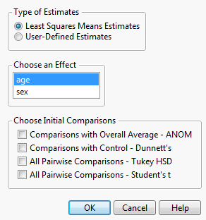
An example of the control window for the Multiple Comparisons option is shown in Launch Window for Least Squares Means Estimates. This example is based on the Big Class.jmp data table, with weight as Y and age, sex, and height as model effects. Two classes of estimates are available for comparisons: Least Squares Means Estimates and User-Defined Estimates.
This option compares least squares means and is available only if there are nominal or ordinal effects in the model. Recall that least squares means are means computed at some neutral value of the other effects in the model. (For a definition of least squares means, see LSMeans Table.) You must select the effect of interest. In Launch Window for Least Squares Means Estimates, Least Squares Means Estimates for age are specified.
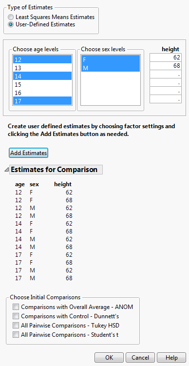
The specification of User-Defined Estimates is illustrated in Launch Window for User-Defined Estimates. Three levels of age and both levels of sex have been selected. Also, two values of height have been manually entered. The Add Estimates button has been clicked, resulting in the listing of all possible combinations of the specified levels. At this point, you can specify more estimates and click the Estimates button again to add them to the list of Estimates for Comparison.
Note: In this section, we will use the term mean to refer to either estimates of least squares means or user-defined estimates.
Shows the t ratio for the significance test.
Gives the p-value for the significance test.
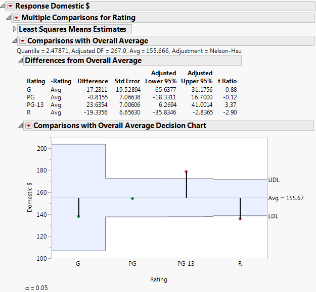
This option compares the means for the specified levels specified to the overall mean for these levels. It displays a table showing confidence intervals for differences from the overall mean and a chart showing decision limits. The method used to make the comparisons is called analysis of means (ANOM) (Nelson, et al., 2005). ANOM is a multiple comparison procedure that controls the joint error rate for all pairwise comparisons to the overall mean. See Comparisons with Overall Average for Ratings for a report based on the Movies.jmp sample data table.
The value of Nelson’s h statistic used in constructing the decision limits.
Specifically, the average least squares mean is a weighted average with weights inversely proportional to the diagonal entries of the matrix  . Here L is the matrix of coefficients used to compute the group least squares means. For a technical definition of least squares means and the average least squares mean, see the GLM Procedure section in the SAS/STAT 9.3 User’s Guide. Search for “Construction of Least Squares Means”.
. Here L is the matrix of coefficients used to compute the group least squares means. For a technical definition of least squares means and the average least squares mean, see the GLM Procedure section in the SAS/STAT 9.3 User’s Guide. Search for “Construction of Least Squares Means”.For user-defined estimates, the average mean is defined similarly. However, in this case, L is the matrix of coefficients used to define the estimates.
|
–
|
Nelson: Provides exact critical values and p-values. Used whenever possible, in particular, when the estimates are uncorrelated.
|
|
–
|
Nelson-Hsu: Provides approximate critical values and p-values based on Hsu’s factor analytical approximation is used (Hsu, 1992). Used when exact values can not be obtained.
|
For technical details, see the GLM Procedure section in the SAS/STAT 9.3 User’s Guide. Search for “Approximate and Simulation-Based Methods”.
Adds columns giving t ratios (t Ratio) and p-values (Prob>|t|) to the Comparisons with Overall Average report. Note that computing exact critical values and p-values for unbalanced designs requires complex integration and can be computationally challenging. When calculations for such a quantile fail, the Sidak quantile is computed but p-values are not available.
Consider the Movies.jmp sample data table. You are interested in whether any of the four Rating categories are unusual in that their mean Domestic $ revenues differ from the overall average revenue. You specify a model with Domestic $ as the response and Type, Rating, and Year as model effects.
|
1.
|
|
2.
|
Select Analyze > Fit Model.
|
|
3.
|
|
4.
|
|
5.
|
Click Run.
|
|
6.
|
|
7.
|
|
8.
|
In the Choose Initial Comparisons list, select Comparisons with Overall Average.
|
|
9.
|
Click OK.
|
|
10.
|
From the Comparisons with Overall Average red triangle menu, select Calculate P-Values.
|
The results shown in Comparisons with Overall Average for Ratings indicate that the least squares means for movies with a Rating of PG-13 and R differ significantly from the overall average in terms of Domestic $.
|
–
|
Dunnett: Provides exact critical values and p-values. Used whenever possible, in particular, when the estimates are uncorrelated.
|
|
–
|
Dunnett-Hsu: Provides approximate critical values and p-values based on Hsu’s factor analytical approximation (Hsu, 1992). Used when exact values can not be obtained.
|
For technical details, see the GLM Procedure section in the SAS/STAT 9.3 User’s Guide. Search for “Approximate and Simulation-Based Methods”.
For each comparison of a group mean to the control mean, this report provides the following details:
Adds columns giving t ratios (t Ratio) and p-values (Prob>|t|) to the Comparisons with Control report. Note that computing exact critical values and p-values for unbalanced designs requires complex integration and can be computationally challenging. When calculations for such a quantile fail, the Sidak quantile is computed but p-values are not available.
The All Pairwise Comparisons option shows either a Tukey HSD All Pairwise Comparisons or Student’s t All Pairwise Comparisons report (Hsu, 1996 and Westfall et al., 2011). Tukey HSD comparisons are constructed so that the significance level applies jointly to all pairwise comparisons. In contrast, for Student’s t comparisons, the significance level applies to each individual comparison. When making several pairwise comparisons using Student’s t tests, the risk that one of the comparisons incorrectly signals a difference can well exceed the stated significance level.
The critical value for the test. Note that, for Tukey HSD, the quantile is  , where q is the appropriate percentage point of the Studentized range statistic.
, where q is the appropriate percentage point of the Studentized range statistic.|
–
|
Tukey: Provides exact critical values and p-values. Used when the means are uncorrelated and have equal variances, or when the design is variance-balanced.
|
|
–
|
Tukey-Kramer: Provides approximate critical values and p-values. Used when exact values can not be obtained.
|
For technical details, see the GLM Procedure section in the SAS/STAT 9.3 User’s Guide. Search for “Approximate and Simulation-Based Methods”.
Both Tukey HSD and Student’s t compare all pairs of levels. For each pairwise comparison, the All Pairwise Differences report shows:
|
•
|
t Ratio - the t ratio for the test of whether the difference is zero
|
|
•
|
Prob > |t| - the p-value for the test
|
This plot, sometimes called a diffogram or a mean-mean scatterplot, displays the confidence intervals for all means pairwise differences. (See All Pairwise Comparisons Scatterplot for User-Defined Comparisons for an example.) Colors indicate which differences are significant.
Use this option to conduct one or more equivalence tests. Equivalence tests are useful when you want to detect differences that are of practical interest. You are asked to specify a threshold difference for group means for which smaller differences are considered practically equivalent. In other words, if two group means differ by this amount or less, you are willing to consider them equivalent.
Once you have specified this value, the Equivalence Tests report appears. The bounds that you have specified are given at the top of the report. The report consists of a table giving the equivalence tests and a scatterplot that displays them. The equivalence tests and confidence intervals are based on Tukey HSD or Student’s t critical values, corresponding to the option that you selected.
The Two One-Sided Tests (TOST) method is used to test for a practical difference between the means (Schuirmann, 1987). Two one-sided pooled-variance t tests are constructed for the null hypotheses that the true difference exceeds the threshold values. If both tests reject, the difference in the means does not statistically exceed either threshold value. Therefore, the groups are considered practically equivalent. If only one or neither test rejects, then the groups might not be practically equivalent.
|
•
|
Lower Bound t Ratio, Upper Bound t Ratio - the lower and upper bound t ratios for the two one-sided pooled-variance significance tests
|
|
•
|
Lower Bound p-Value, Upper Bound p-value - p-values corresponding to the lower and upper bound t ratios
|
 confidence interval for the difference in the means.
Using colors, this scatterplot indicates which means are practically equivalent and which are not as determined by the equivalence test. (See Equivalence Tests Scatterplot.)
 confidence interval for a pairwise comparison. The coordinates of the point on the line segment are the means for the corresponding groups. Placing your cursor over one of these points displays a tooltip indicating the groups being compared and the estimated difference. When a line segment is entirely contained within the diagonal band, it follows that the means are practically equivalent.
Consider the Movies.jmp sample data table. You are interested in Domestic $ differences for action and drama movies across two Rating categories, PG-13 and R, in the year 1998.
|
1.
|
|
2.
|
Select Analyze > Fit Model.
|
|
3.
|
|
4.
|
|
5.
|
Click Run.
|
|
6.
|
|
7.
|
From the Type of Estimates list, click User-Defined Estimates.
|
|
10.
|
In the list entitled Year, enter the year 1998.
|
|
11.
|
Click Add Estimates. Note that all possible combinations of the levels you specified are now displayed beneath the Add Estimates button.
|
|
12.
|
In the Choose Initial Comparisons list, select All Pairwise Comparisons - Tukey HSD.
|
|
13.
|
Click OK.
|
The All Pairwise Differences report indicates that three of the six pairwise comparisons are significant. The All Pairwise Comparisons Scatterplot, shown in All Pairwise Comparisons Scatterplot for User-Defined Comparisons, shows the confidence intervals for these comparisons in red. Also shown is the tooltip for one of these intervals, indicating that the interval compares Action, Rating R movies to Drama, Rating PG-13 movies, and that the mean difference in Domestic $ is -53.58.
|
14.
|
|
16.
|
Click OK.
|
TOST tests are conducted to determine which movie categories are equivalent, given that you consider categories that differ by less than 50 in units of Domestic $ to be equivalent. The Equivalence Tests Scatterplot (Equivalence Tests Scatterplot) indicates that two pairs of movie categories can be considered equivalent.