You can create a formula that calculates probabilities and quantiles for statistical distributions like beta, Chi-square, F, gamma, normal, Student’s t, Weibull distributions, Tukey HSD, and so on. See Probability Functions in the JSL Syntax Reference for details about syntax.
Accepts an argument from the range of values for the standard normal distribution, which is all real numbers. It returns the value of the standard normal probability density function (pdf) for the argument. For example, you can create a column of values (X) with the formula count(-3, 3, nrow()). In a second column, insert the formula Normal Density(X) to generate density values. Then select Graph > Graph Builder to plot the normal density by X.
Accepts an argument x from the range of values for the standard normal distribution, which is all real numbers. It returns the probability that an observation from the standard normal distribution is less than or equal to x. For example, the expression Normal Distribution(1.96) returns 0.975, the probability that an observation from the standard normal distribution is less than or equal to the 1.96th quantile. Also, you can specify mean and standard deviation parameters to obtain probabilities from nonstandard normal distributions. The Normal Distribution function is the inverse of the Normal Quantile function.
Accepts a probability argument p, and returns the pth quantile from the standard normal distribution. For example, the expression Normal Quantile(0.975) returns the 97.5% quantile from the standard normal distribution, which evaluates as 1.96. Also, you can specify parameter values for the mean and standard deviation to obtain quantiles from nonstandard normal distributions. The Normal Quantile function is the inverse of the Normal Distribution function.
Requires three arguments: quantile argument and the shape parameters alpha and beta. A threshold parameter (θ) and a scale parameter (σ > 0) are additional arguments. It returns the value of the beta probability density function (pdf) for the given arguments. The beta density is useful for modeling the probabilistic behavior of random variables such as proportions constrained to fall in the interval [0, 1].
The beta distribution has two shape parameters: α > 0 and β > 0. A threshold parameter (θ) and a scale parameter (σ) are additional arguments, where θ≤ x ≤θ + σ. The default value for θ is 0. The default value for σ is 1.
Accepts a probability argument, p, and shape and scale parameters, α > 0 and β > 0. It returns the pth quantile from the standard beta distribution. The beta quantile function is the inverse of the beta distribution function.
Accepts an argument x, which can be any real number, and optional arguments center and scale. If you do not specify values for the optional arguments, the function returns the value at x of the Cauchy probability density function (pdf) for a distribution with median 0 and third quartile 1.
If you specify values for center and scale, the function returns the value at x of the Cauchy probability function, characterized as follows:
|
•
|
The optional parameter center is the median of the distribution.
|
|
•
|
The optional parameter scale is half of the interquartile range, namely, half of the difference between the 0.75 and 0.25 quantiles.
|
Accepts an argument x, which can be any real number, and optional arguments center and scale. If you do not specify values for the optional arguments, the function returns the value at x of the Cauchy cumulative distribution function (cdf) for a distribution with median 0 and third quartile 1. If you specify values for center and scale, the function returns the value at x of the cumulative distribution function for the Cauchy distribution with median given by center and interquartile range given by twice the scale.
Accepts an argument prob, which can be any number between 0 and 1, and optional arguments center and scale. If you do not specify values for the optional arguments, the function returns the pth quantile, where p = prob, of a Cauchy distribution with median 0 and third quartile 1. If you specify values for center and scale, the function returns the pth quantile of a Cauchy distribution with median given by center and interquartile range given by twice the scale.
Accepts a response argument (range of x values) and three parameter arguments: a quantile, a degrees of freedom, and a noncentrality parameter. It returns the probability that an observation from the Chi-squared distribution with the specified noncentrality parameter and degrees of freedom is less than or equal to the given quantile. For example, the expression ChiSquare Distribution(11.264, 5) returns the probability that an observation from the Chi-squared distribution centered at 0 with 5 degrees of freedom is less than or equal to 11.264. The expression evaluates as 0.95361.
Furthermore, the ChiSquare Distribution function accepts integer and noninteger degrees of freedom. It is centered at 0 by default. The ChiSquare Distribution function is the inverse of the ChiSquare Quantile function.
Returns the noncentrality parameter nc such that probability is equal to the probability that a Chi-square distributed random variable with df degrees of freedom is less than x.
Returns the quantile from a Chi-square distribution, the value for which the probability is p that a random value would be lower.
Accepts three arguments: a probability p, a degrees of freedom, and a noncentrality parameter. It returns the pth quantile from the Chi-squared distribution with the specified noncentrality parameter and degrees of freedom. For example, the expression ChiSquare Quantile(.95, 3.5, 4.5) returns the 95% quantile from the Chi-squared distribution centered at 4.5 with 3.5 degrees of freedom. The expression evaluates as 17.50458.
The ChiSquare Quantile function accepts integer and noninteger degrees of freedom. It is centered at 0 by default. The ChiSquare Quantile function is the inverse of the ChiSquare Distribution function.
Returns the p-value from Dunnett’s multiple comparison test.
Accepts a quantile argument from the range of values for the F-distribution, numerator and denominator degrees of freedom arguments, and an optional noncentrality parameter. It returns the value of the F-density function (pdf) for the arguments.
Accepts four arguments: a quantile, a numerator and denominator degrees of freedom, and a noncentrality parameter. It returns the probability that an observation from the F-distribution with the specified noncentrality parameter and degrees of freedom is less than or equal to the given quantile. For example, the expression F Distribution(3.32, 2, 3) returns the probability that an observation from the central F-distribution with 2 degrees of freedom in the numerator and 3 degrees of freedom in the denominator is less than or equal to 3.32. The expression evaluates as 0.82639.
The F-distribution function accepts integer and noninteger degrees of freedom. By default, the non-central parameter is set to 0. The F-distribution function is the inverse of the F Quantile function.
Returns the log of 1 - F-distribution.
Returns the log of the F-distribution.
Solves the noncentrality such that prob=F-distribution (x, ndf, ddf, nc).
The F Power function calculates the power from a given situation that involves an F-test or t-test, and the F Sample Size function computes the sample size. The arguments are the values that you specify for computation of a prospective power analysis. (These functions perform the same computations as if you selected DOE > Sample Size and Power. See Prospective Sample Size and Power in the Design of Experiments Guide for a discussion of power and sample size.) The arguments include:
|
•
|
alpha The significance level that you are willing to tolerate (often 0.05).
|
|
•
|
dfh The hypothesis degrees of freedom. It is one (1) for a t-test.
|
|
•
|
|
•
|
SquaredSize The squared effect size scaled by the error variance, which is used for making the noncentrality argument for the F-distribution. For this argument, use squared size = Δ2/σ2 where σ2 is the error variance. That is, use:
|
 for a one-sample t-test
 for a two-sample t-test
 for a
for a |
•
|
n (found only in the F Power function) The total number of observations (runs, experimental units, or samples) you expect to have. Power (in the F Sample Size function) is the probability that you want to have of declaring a significant result.
|
Accepts four arguments: a probability p, a numerator and denominator degrees of freedom, and a noncentrality parameter. It returns the pth quantile from the F-distribution with the specified noncentrality parameter and degrees of freedom. For example, the expression F Quantile(0.95, 2, 10, 0) returns the 95% quantile from the F-distribution centered at 0 with 2 degrees of freedom in the numerator and 10 degrees of freedom in the denominator. The expression evaluates as 4.1028.
The F Quantile function accepts integer and noninteger degrees of freedom. By default, the non-central parameter is set to 0. The F Quantile function is the inverse of the F Distribution function.
Returns the probability that a Fréchet distribution with location mu and scale sigma is less than x.
Returns the quantile associated with a cumulative probability p for a Fréchet distribution with location mu and scale sigma.
Requires a quantile argument. Also accepts an optional alpha shape parameter, which must be greater than zero and defaults to 1. A scale parameter b, which must be greater than zero and defaults to 1, is optional. A threshold parameter, which must be in the range -∞ < θ < +∞ and defaults to zero, is optional.
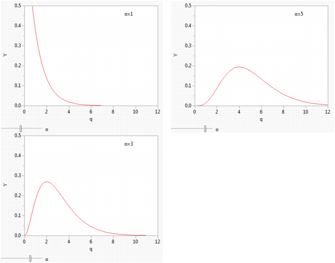
Gamma Density Example shows the shape of gamma probability density functions for shape parameters of 1, 3, and 5. The standard gamma density function is strictly decreasing when α (shape) ≤1. When α > 1 the density function begins at zero when x is θ, increases to a maximum, and then decreases.
Is based on the standard gamma function, and accepts a single argument with a quantile value. The shape, scale, and threshold parameters are optional, with defaults as described previously in the discussion of the Gamma Density function. It returns the probability that an observation from a standard gamma distribution is less than or equal to the specified x. The Gamma Distribution function is the inverse of Gamma Quantile function.
Accepts a probability argument p, and returns the pth quantile from the standard gamma distribution with the shape parameter that you specify. The Gamma Quantile function is the inverse of the Gamma Distribution function.
Returns the density at x of a GenGamma probability distribution with parameters mu, sigma, and lambda.
Returns the quantile from a GenGamma distribution, the value for which the probability is p that a random value would be lower. mu, sigma, and lambda are parameters, respectively.
Returns the density or pdf at a particular quantile q of a generalized logarithm distribution with location mu, scale sigma, and shape lambda. When the shape parameter is equal to zero, the distribution reduces to a Lognormal(mu, sigma).
Returns the probability or cdf that a generalized logarithm distributed random variable is less than q. When the shape parameter is equal to zero, the distribution reduces to a Lognormal(mu, sigma).
Returns the quantile, the value for which the probability is p that a random value would be lower. When the shape parameter is equal to zero, the distribution reduces to a Lognormal(mu, sigma).
Returns the probability that a Johnson Sb-distributed random variable is less than x. There are four optional arguments: gamma, delta, theta, and sigma. For a description of the Johnson Sb distribution and these parameters, see Johnson Sb Distribution(q, gamma, delta, theta, sigma) the JSL Syntax Reference book.
Returns the pth quantile of the Johnson Sb distribution. There are four optional arguments: gamma, delta, theta, and sigma. For a description of the Johnson Sb distribution and these parameters, see Johnson Sb Quantile(p, gamma, delta, theta, sigma) the JSL Syntax Reference book.
Returns the density at x of a Johnson Sb distribution. There are four optional arguments: gamma, delta, theta, and sigma. For a description of the Johnson Sb distribution and these parameters, see Johnson Sl Density(q, gamma, delta, theta, sigma) the JSL Syntax Reference book.
Returns the probability that a Johnson Sl-distributed random variable is less than x. There are four optional arguments: gamma, delta, theta, and sigma. For a description of the Johnson Sl distribution and these parameters, see Johnson Sl Distribution(q, gamma, delta, theta, sigma) the JSL Syntax Reference book.
Returns the pth quantile of the Johnson Sl distribution. There are four optional arguments: gamma, delta, theta, and sigma. For a description of the Johnson Sl distribution and these parameters, see Johnson Sl Quantile(p, gamma, delta, theta, sigma) the JSL Syntax Reference book.
Returns the density at x of a Johnson Sl distribution. There are four optional arguments: gamma, delta, theta, and sigma. For a description of the Johnson Sl distribution and these parameters, see Johnson Sl Density(q, gamma, delta, theta, sigma) the JSL Syntax Reference book.
Returns the probability that a Johnson Su-distributed random variable is less than x. There are four optional arguments: gamma, delta, theta, and sigma. For a description of the Johnson Su distribution and these parameters, see Johnson Su Distribution(q, gamma, delta, theta, sigma) the JSL Syntax Reference book.
Returns the pth quantile of the Johnson Su distribution. There are four optional arguments: gamma, delta, theta, and sigma. For a description of the Johnson Su distribution and these parameters, see Johnson Su Quantile(p, gamma, delta, theta, sigma) the JSL Syntax Reference book.
Returns the density at x of a Johnson Su distribution. There are four optional arguments: gamma, delta, theta, and sigma. For a description of the Johnson Su distribution and these parameters, see Johnson Su Density(q, gamma, delta, theta, sigma) the JSL Syntax Reference book.
Returns the density at x of the largest extreme value distribution with location mu and scale sigma.
Returns the probability that the largest extreme value distribution with location mu and scale sigma is less than x.
Returns the quantile associated with a cumulative probability p of the largest extreme value distribution with location mu and scale sigma.
Returns the quantile from a LogGenGamma distribution, the value for which the probability is p that a random value would be lower. mu, sigma, and lambda are parameters, respectively.
Returns the probability that the logistic distribution with location mu and scale sigma is less than x.
Returns the quantile associated with a cumulative probability p of the logistic distribution with location mu and scale sigma.
Returns the probability that the loglogistic distribution with location mu and scale sigma is less than x.
Returns the quantile associated with a cumulative probability p of the loglogistic distribution with location mu and scale sigma.
Returns the probability that the lognormal distribution with location mu and scale sigma is less than x.
Returns the quantile associated with a cumulative probability p of a lognormal distribution with location mu and scale sigma.
Computes the probability that an observation is less than or equal to (x,y) with correlation coefficient r where the observation is marginally normally distributed. You can specify the mean and standard deviation for the X and Y coordinates of the observation. The default values are 0 for both means and 1 for both standard deviations.
Returns the density at q of a normal mixture distribution with group means mean, group standard deviations stdev, and group probabilities probability. The mean, stdev, and probability arguments are all vectors of the same size.
Returns the probability that a normal mixture distributed variable with group means mean, group standard deviations stdev, and group probabilities probability is less than q. The mean, stdev, and probability arguments are all vectors of the same size.
Returns the quantile, the values for which the probability is p that a random value would be lower. The mean, stdev, and probability arguments are all vectors of the same size.
Returns the probability that the smallest extreme distribution with location mu and scale sigma is less than x.
Returns the quantile associated with a cumulative probability p of the smallest extreme distribution with location mu and scale sigma.
Accepts a quantile argument from the range of values for the t-distribution, a degrees of freedom argument, and an optional noncentrality parameter. It returns the value of the t-density function (pdf) for the arguments. To compare a t-density with 5 df with a standard normal distribution, you can create a column of quantile values (X) with the formula count(-3, 3, nrow()). In a second column, insert the formula t Density(X, 5). In a third column, insert the formula Normal Density(X). Then select Graph > Graph Builder to plot the t-density and the normal density by X. You will see that the t-density has slightly more spread than the normal.
Accepts three arguments: a quantile, a degrees of freedom, and a noncentrality parameter. It returns the probability that an observation from the Student’s t-distribution with the specified noncentrality parameter and degrees of freedom is less than or equal to the given quantile. For example, the expression t Distribution(.9, 5) returns the probability that an observation from the Student’s t-distribution centered at 0 with 5 degrees of freedom is less than or equal to 0.9. The expression is evaluated as 0.79531. t-distribution accepts integer and noninteger degrees of freedom. It is centered at 0 by default, but you can enter a value for the noncentrality parameter. The t Quantile function is the inverse of the t Distribution function.
Solves the noncentrality such that prob=T Distribution (x, df, nc).
Accepts three arguments: a probability p, a degrees of freedom, and a noncentrality parameter. It returns the pth quantile from the Student’s t-distribution with the specified noncentrality parameter and degrees of freedom. For example, the expression Student’s t Quantile(.95, 2.5) returns the 95% quantile from the Student’s t-distribution centered at 0 with 2.5 degrees of freedom. The expression evaluates as 2.558219. The t Quantile function is the inverse of the t Distribution function. This function also accepts integer and noninteger degrees of freedom. It is centered at 0 by default, but you have the option to enter a value for the noncentrality parameter. The t Distribution function is the inverse of the t Quantile function.
Accepts a probability argument 1-alpha, and returns the 1-alphath quantile from Tukey’s HSD test for the parameters that you specify. The alpha argument is the significance level that you want. nGroups is the number of groups in a study. dfe is the error degrees of freedom (based on the total study sample). This is the quantile used to calculate least significant difference in Tukey’s multiple comparisons test.
Returns the p-value from Tukey’s HSD multiple comparisons test.
Accepts a quantile argument from the range of values for the Weibull distribution, and optional shape, scale, and threshold arguments. The density function for a Weibull distribution with shape parameter β, scale parameter α, and threshold parameter θ is given in Weibull, Weibull with Threshold, and Extreme Value in the Basic Analysis book. The Weibull Density function returns the value of the probability density function (pdf) for the corresponding Weibull distribution.
Accepts a quantile argument x from the range of values for the Weibull distribution, and optional shape, scale, and threshold arguments. The distribution function for a Weibull distribution with shape parameter β, scale parameter α, and threshold parameter θ is given in the Basic Analysis book. The Weibull Distribution function returns the probability that an observation is less than or equal to the specified x for the Weibull distribution with the shape, scale, and threshold parameters that you specified. The Weibull Distribution function is the inverse of Weibull Quantile function.
The Weibull distribution has different shapes depending on the values of α (a scale parameter that affects the x direction) and β (a shape parameter). It often provides a good model for estimating the length of life, especially for mechanical devices and in biology. The two-parameter Weibull is the same as the three-parameter Weibull with a threshold of zero.
Accepts a probability argument p, and returns the pth quantile from the Weibull distribution with the shape, scale, and threshold parameters that you specify. The Weibull Quantile function is the inverse of the Weibull Distribution function.