The Normal fitting option estimates the parameters of the normal distribution. The normal distribution is often used to model measures that are symmetric with most of the values falling in the middle of the curve. Select the Normal fitting for any set of data and test how well a normal distribution fits your data.
|
•
|
μ (the mean) defines the location of the distribution on the x-axis
|
|
•
|
σ (standard deviation) defines the dispersion or spread of the distribution
|
The standard normal distribution occurs when  and
and  . The Parameter Estimates table shows estimates of μ and σ, with upper and lower 95% confidence limits.
and . The Parameter Estimates table shows estimates of μ and σ, with upper and lower 95% confidence limits.pdf: 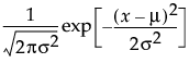 for
for  ;
;  ; 0 < σ
for ; ; 0 < σThe LogNormal fitting option estimates the parameters μ (scale) and σ (shape) for the two-parameter lognormal distribution. A variable Y is lognormal if and only if  is normal. The data must be greater than zero.
is normal. The data must be greater than zero.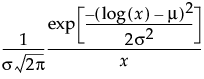 for
for  ;
;  ; 0 <
; 0 < 
The Weibull distribution has different shapes depending on the values of α (scale) and β (shape). It often provides a good model for estimating the length of life, especially for mechanical devices and in biology. The Weibull option is the same as the Weibull with threshold option, with a threshold (θ) parameter of zero. For the Weibull with threshold option, JMP estimates the threshold as the minimum value. If you know what the threshold should be, set it by using the Fix Parameters option. See Fit Distribution Options.
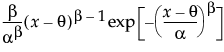 for
for 
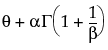
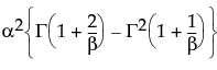
 is the Gamma function.
The Extreme Value distribution is a two parameter Weibull (α, β) distribution with the transformed parameters δ = 1 / β and λ = ln(α).
The Exponential distribution is a special case of the two-parameter Weibull when β = 1 and α = σ, and also a special case of the Gamma distribution when α = 1.
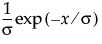 for 0 <
Devore (1995) notes that an exponential distribution is memoryless. Memoryless means that if you check a component after t hours and it is still working, the distribution of additional lifetime (the conditional probability of additional life given that the component has lived until t) is the same as the original distribution.
The Gamma fitting option estimates the gamma distribution parameters, α > 0 and σ > 0. The parameter α, called alpha in the fitted gamma report, describes shape or curvature. The parameter σ, called sigma, is the scale parameter of the distribution. A third parameter, θ, called the Threshold, is the lower endpoint parameter. It is set to zero by default, unless there are negative values. You can also set its value by using the Fix Parameters option. See Fit Distribution Options.
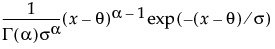 for
for  ; 0 <
; 0 < |
•
|
The standard gamma distribution has σ = 1. Sigma is called the scale parameter because values other than 1 stretch or compress the distribution along the x-axis.
|
|
•
|
 distribution occurs when
 |
•
|
 . When
  , the density function begins at zero, increases to a maximum, and then decreases.
The standard beta distribution is useful for modeling the behavior of random variables that are constrained to fall in the interval 0,1. For example, proportions always fall between 0 and 1. The Beta fitting option estimates two shape parameters, α > 0 and β > 0. There are also θ and σ, which are used to define the lower threshold as θ, and the upper threshold as θ + σ. The beta distribution has values only for the interval defined by 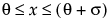 . The θ is estimated as the minimum value, and σ is estimated as the range. The standard beta distribution occurs when θ = 0 and σ = 1.
. The θ is estimated as the minimum value, and σ is estimated as the range. The standard beta distribution occurs when θ = 0 and σ = 1.Set parameters to fixed values by using the Fix Parameters option. The upper threshold must be greater than or equal to the maximum data value, and the lower threshold must be less than or equal to the minimum data value. For details about the Fix Parameters option, see Fit Distribution Options.
 for
for  ; 0 <
; 0 < 
 is the Beta function.
The Normal Mixtures option fits a mixture of normal distributions. This flexible distribution is capable of fitting multi-modal data.
Fit a mixture of two or three normal distributions by selecting the Normal 2 Mixture or Normal 3 Mixture options. Alternatively, you can fit a mixture of k normal distributions by selecting the Other option. A separate mean, standard deviation, and proportion of the whole is estimated for each group.
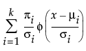

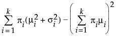
where μi, σi, and πi are the respective mean, standard deviation, and proportion for the ith group, and  is the standard normal pdf.
is the standard normal pdf.The Smooth Curve option fits a smooth curve using nonparametric density estimation (kernel density estimation). The smooth curve is overlaid on the histogram and a slider appears beneath the plot. Control the amount of smoothing by changing the kernel standard deviation with the slider. The initial Kernel Std estimate is calculated from the standard deviation of the data.
 .
.
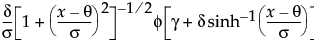 for
for  ; 0 <
; 0 < 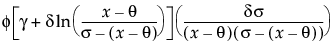 for
for 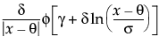 for
for  is the standard normal pdf.
Note: The parameter confidence intervals are hidden in the default report. Parameter confidence intervals are not very meaningful for Johnson distributions, because they are transformations to normality. To show parameter confidence intervals, right-click in the report and select Columns > Lower 95% and Upper 95%.
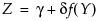
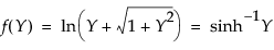
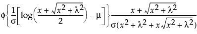
This distribution is useful for fitting data that are rarely normally distributed and often have non-constant variance, like biological assay data. The Glog distribution is described with the parameters μ (location), σ (scale), and λ (shape).
 ; 0 <
; 0 < 
 ~ N(0,1), then
Note: The parameter confidence intervals are hidden in the default report. Parameter confidence intervals are not very meaningful for the GLog distribution, because it is a transformation to normality. To show parameter confidence intervals, right-click in the report and select Columns > Lower 95% and Upper 95%.
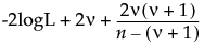
In the Compare Distributions report, the ShowDistribution list is sorted by AICc in ascending order.
|
–
|
n is the sample size
|
|
–
|
ν is the number of parameters
|