Repeated Measures Example

Consider the Cholesterol Stacked.jmp sample data table. A study was performed to test two new cholesterol drugs against a control drug. Twenty patients with high cholesterol were randomly assigned to each of four treatments (the two experimental drugs, the control, and a placebo). Each patient’s total cholesterol was measured at six times during the study: the first day in April, May, and June in the morning and afternoon. You are interested in whether either of the new drugs is effective at lowering cholesterol and in whether time and treatment interact.

Background

Two methods have historically been used to analyze such a design:

•

Multivariate analysis of variance (MANOVA)

•

A split-plot in time univariate analysis of variance (ANOVA) with either the Huynh-Feldt (1976) or Greenhouse-Geisser (1959) correction

Both of these options are available using the MANOVA personality in Fit Model. These two options are the two extremes for modeling the covariance structure. The MANOVA analysis assumes an unstructured covariance structure where all variances and covariances are estimated individually. The independent split-plot in time analysis assumes that all errors are independent. In the Gaussian data case, this is equivalent to assuming a compound symmetry covariance structure.

These two models can result in vastly different conclusions about the treatment effects. When you assume a complex covariance structure, information in the data is used to estimate the covariance parameters. If you fit too many covariance parameters, you run the risk of overfitting your model. When you model repeated measures data, you must find a covariance structure that balances these issues.

•

When the model is overfit, the power to detect differences is smaller than if you were to assume a less complex covariance structure.

•

When the model is underfit, Type I error control is lost. In some cases, this leads to inflated rejection rates. In other cases, decreased rejection rates occur due to inflated variance.

Covariance Structures

The Mixed Model personality fits a variety of covariance structures. For repeated measures in time, both the Toeplitz covariance structure and the first-order autoregressive (AR(1)) covariance structures often provide appropriate correlation structures. These structures allow for correlated observations without overfitting the model. The AR(1) assumes a common variance parameter, whereas the Toeplitz covariance matrix with unequal variances estimates unique variances for each unit of the repeated measure variable. See Repeated Covariance Structure Requirements.

In this example, you fit the four covariance structures. The number of observation times, J, is equal to six.

•

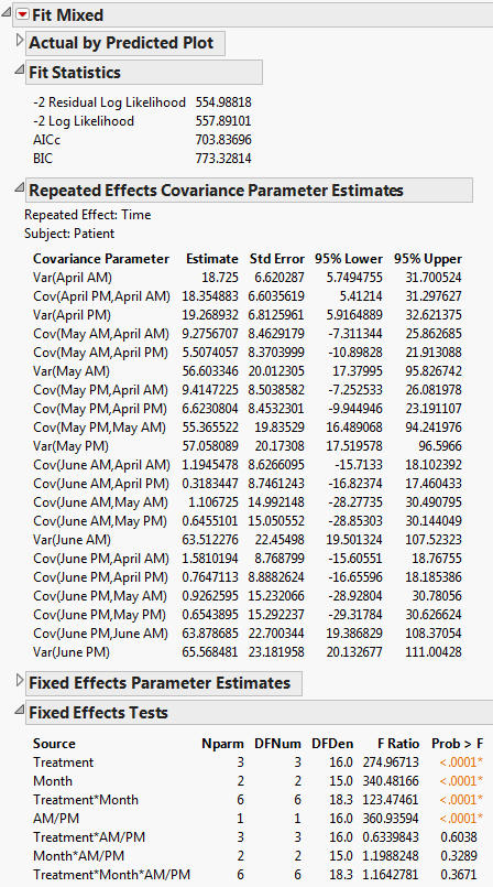
Covariance Structure: Unstructured. The Unstructured model fits all covariance parameters, J(J+1)/2 in total. In this example, the model fits 21 variances.

•

Covariance Structure: Residual. The Residual model is equivalent to the usual variance components structure. In this example, the model fits two variances.

•

Covariance Structure: Toeplitz. The Toeplitz model fits 2J-1 covariance parameters. In this example, the model fits 11 variances.

•

Covariance Structure: AR(1). This model fits two covariance parameters. One parameter determines the variance and the other determines how the covariance changes with time.

You use AICc to evaluate model fits. The BIC criterion can also be used. In this case, the same model is chosen by both criteria. You select a best covariance structure and then continue to do additional analysis:

•

Further Analysis Using AR(1) Structure

•

Regression Model for AR(1) Model Example

Tip: Leave the Fit Model launch window open as you work through this example.

Data Structure

The Cholesterol.jmp data table is in a format that is typically used for recording repeated measures data. To use the Mixed Model personality to analyze these data, each cholesterol measurement needs to be in its own row, as in Cholesterol Stacked.jmp. To construct Cholesterol Stacked.jmp, the data in Cholesterol.jmp were stacked using Tables > Stack.

The Days column in the stacked table was constructed using a formula. The Days column gives the number days into the study when the cholesterol measurement was taken. Its modeling type is continuous. This is necessary because the AR(1) covariance structure requires the repeated effect be continuous.

Covariance Structure: Unstructured

Begin by fitting a model using an Unstructured covariance structure.

Select Help > Sample Data Library and open Cholesterol Stacked.jmp.

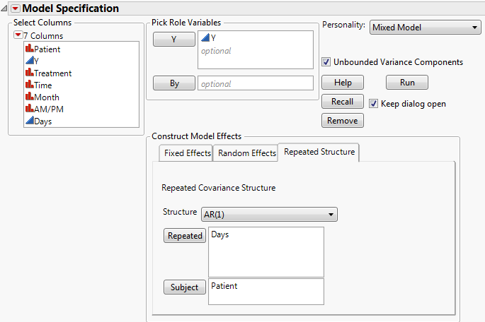
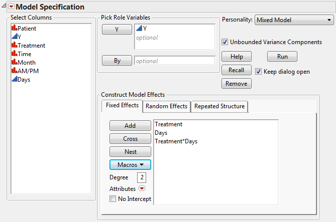
Select Analyze > Fit Model.

Select Keep dialog open so that you can return to the launch window in the next example.

Select Y and click Y.

Select Mixed Model from the Personality list.

Select Treatment, Month, and AM/PM, and then select Macros > Full Factorial.

Fit Model Launch Window Showing Completed Fixed Effects Tab

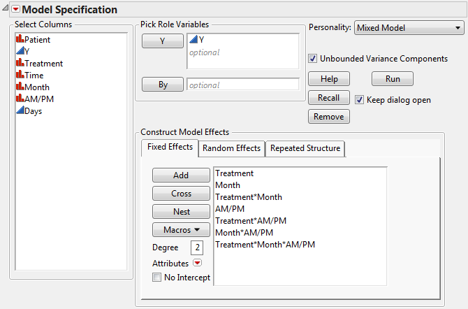
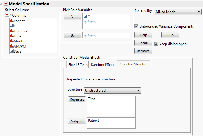
Select the Repeated Structure tab.

Select Unstructured from the Structure list.

Select Time and click Repeated. The Repeated column defines the repeated measures within a subject.

10.

Select Patient and click Subject.

Note: The Unstructured covariance model does not allow the repeated structure variables to assume duplicate values. Suppose that, in this example, the subject was nested within treatment, and that the patients had been numbered using the values 1, 2, 3, 4, and 5 within each treatment. A warning would be given when you run this analysis. You would need to renumber the patients to have different identifiers for each value of the Repeated variable. Or you would need to create a column in the data table that represents nesting within treatment and enter this effect as Subject.

Fit Model Launch Window Showing Completed Repeated Structure Tab

11.

Click Run.

The Fit Mixed report is shown in Fit Mixed Report - Unstructured Covariance Structure. Because you want to compare your three models using AICc or BIC, you are interested in the Fit Statistics report. The AICc for the unstructured model is 703.84.

The Repeated Effects Covariance Parameter Estimates report shows estimates of all 21 covariance parameters. As you would expect, observations taken closer in time have higher covariance than those farther apart. Also, variance increases with time.

Fit Mixed Report - Unstructured Covariance Structure

Covariance Structure: Residual

The Residual covariance structure is appropriate when you fit a split-plot model.

Complete step 1 through step 7 in Covariance Structure: Unstructured.

On the Repeated Structure tab, select Residual from the Structure list.

If you are continuing from the previous example, remove Time and Patient.

Otherwise, a warning appears: “Repeated columns and subject columns are ignored when the Residual covariance structure is selected.” You are given the option to click OK to continue the analysis.

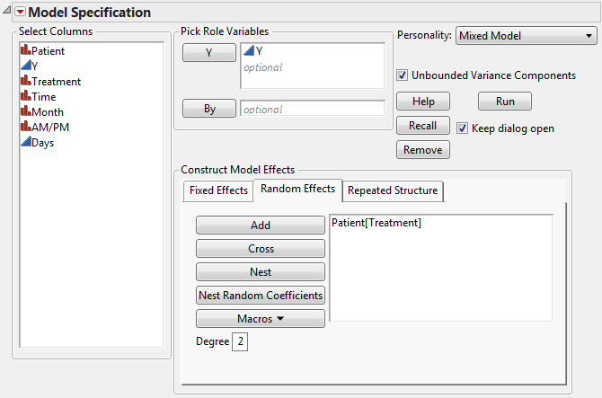
Select the Random Effects tab.

Select Patient and click Add.

Select Patient in the Random Effects area, select the Treatment column, and then click Nest.

Fit Model Launch Window Showing Completed Random Effects Tab

Click Run.

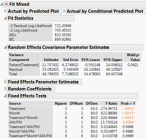
The Fit Mixed report is shown in Fit Mixed Report - Residual Error Covariance Structure. The Fit Statistics report shows that the AICc for the Residual model is 832.55, as compared to 703.84 for the Unstructured model.

The estimates of the two covariance parameters are shown in the Random Effects Covariance Parameter Estimates report. These are estimates of the variance of Patient within Treatment, and of the Residual variance.

Fit Mixed Report - Residual Error Covariance Structure

Covariance Structure: Toeplitz

Fit the model using the Toeplitz Unequal Variances structure.

Complete step 1 through step 6 in Covariance Structure: Unstructured.

If you are continuing from the previous example, select Patient[Treatment] on the Random Effects tab and then click Remove.

If you include both random effects and repeated effects, there is often insufficient data to estimate both effects.

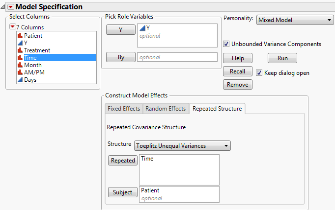
Select the Repeated Structure tab.

Select Toeplitz Unequal Variances from the Structure list.

Select Time and click Repeated.

Select Patient and click Subject.

Fit Model Launch Window Showing Completed Repeated Structure Tab

Click Run.

Fit Mixed Report - Toeplitz Unequal Variances Structure

Note: The Mixed Models personality in JMP reports correlations, whereas PROC MIXED in SAS reports covariances.

The Fit Statistics report shows that the AICc for the Toeplitz with Unequal Variances model is 788.03. Compare this number to 832.55 for the Residual Model and 703.84 for the Unstructured model.

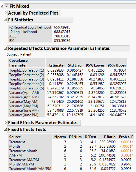
The Toeplitz Unequal Variances structure requires the estimation of eleven covariance parameters. These estimates are shown in the Repeated Effects Covariance Parameter Estimates report. The Toeplitz correlation estimates are shown, followed by the variance estimates for each time point. See Repeated Measures for information about how this matrix is parameterized.

Covariance Structure: AR(1)

Finally, fit the AR(1) structure.

Complete step 1 through step 6 in Covariance Structure: Unstructured.

If you are continuing from the previous example, select Time in the Repeated box and then click Remove.

AR(1) requires a continuous variable for the repeated value.

Select AR(1) from the Structure list.

Select Days and click Repeated.

Fit Model Launch Window Showing Completed Repeated Structure Tab

Click Run.

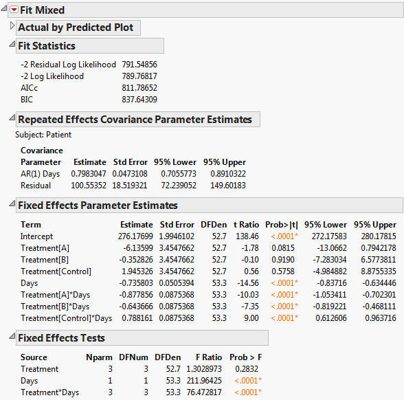
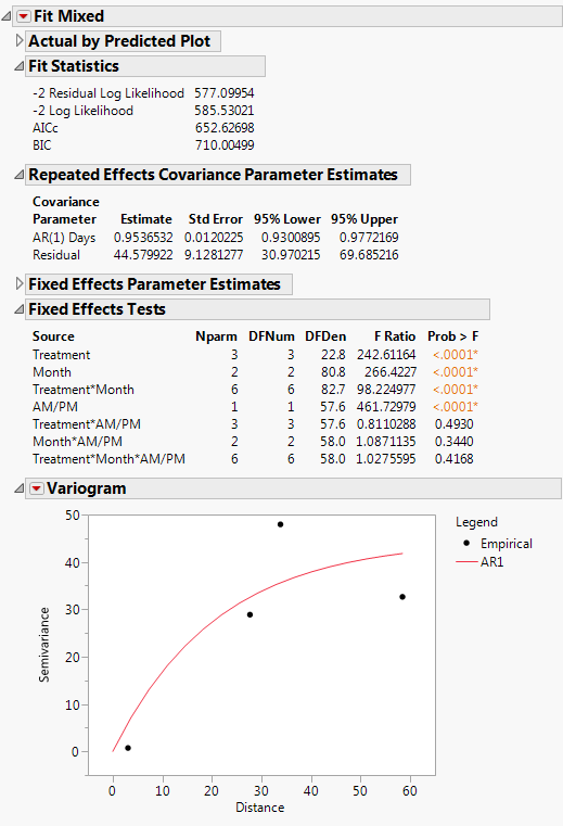
The Fit Mixed report is shown in Fit Mixed Report - AR(1) Covariance Structure. The Fit Statistics report shows that the AICc for the AR(1) model is 652.63. Compare this number to 832.55 for the Residual model, 703.84 for the Unstructured model, and 788.03 for the Toeplitz Unequal Variances model. Based on the AICc criterion, the AR(1) model is the best of the four models.

The AR(1) structure requires the estimation of two covariance parameters. These estimates are shown in the Repeated Effects Covariance Parameter Estimates report. The AR(1) Days parameter estimate is an estimate of ρ, the correlation parameter in the AR(1) structure.

The Variogram plot shows the empirical semivariances and the curve for the AR(1) model. Since there are only five nonzero values for Days, only four distance classes are possible and only four points are shown. The AR(1) structure seems appropriate. To explore other structures, select options from the red triangle menu next to Variogram. For more information about Variogram options, see Variogram.

Fit Mixed Report - AR(1) Covariance Structure

Further Analysis Using AR(1) Structure

Because the AR(1) model gives the best fit, you adopt it as your model and proceed with your analysis. The Fixed Effects Tests report indicates that there is a significant interaction between Treatment and Month as well as a main effect of AM/PM. Here, we explore these significant effects.

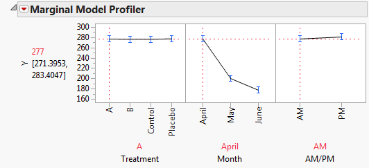
Click the red triangle next to Fit Mixed and select Marginal Model Inference > Profiler.

The Marginal Model Profiler report (Marginal Profiler Plot for Treatment A) enables you to see the effect on cholesterol levels (Y) for various settings of Treatment, Month, and AM/PM.

In the plot for Month, drag the vertical dotted red line from April to May and then to June.

Notice that the predicted AM measurements for Y decrease over the three months from a mean of 277.4 in April to a mean of 177.7 in June.

In the plot for Treatment, drag the vertical dotted red line from A to B.

By dragging the line in the plot for Month from April to June, you see that, for Treatment B, the predicted AM mean for Y decreases from 276.8 in April to 191.2 in June.

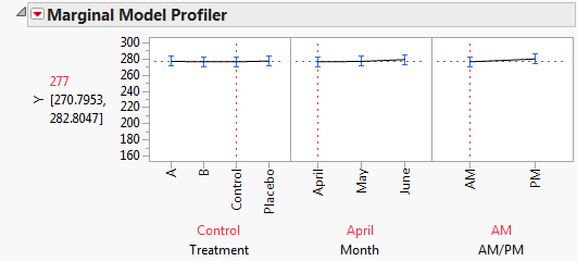
In the plot for Treatment, drag the vertical dotted line to Control and then to Placebo.

Notice that when you set Treatment to Control or Placebo, you see virtually no change over the three months (Marginal Profiler Plot for Control).

Next, you explore the effect of AM/PM.

Set Treatment and Month to all twelve combinations of their levels by dragging the vertical red lines.

For all twelve combinations, the predicted cholesterol level is consistently higher in the afternoon than in the morning, demonstrating the main effect.

Note that Treatment A seems to result in lower cholesterol readings in May than Treatment B does. If this effect is significant, it might indicate that Treatment A acts more quickly than B. The next section, Compare All Treatments in June, shows you how to evaluate the treatments.

Marginal Profiler Plot for Treatment A

Marginal Profiler Plot for Control

Compare All Treatments in June

The study is conducted over the months of April, May, and June. You are interested in which treatments differ on the PM measurement in June.

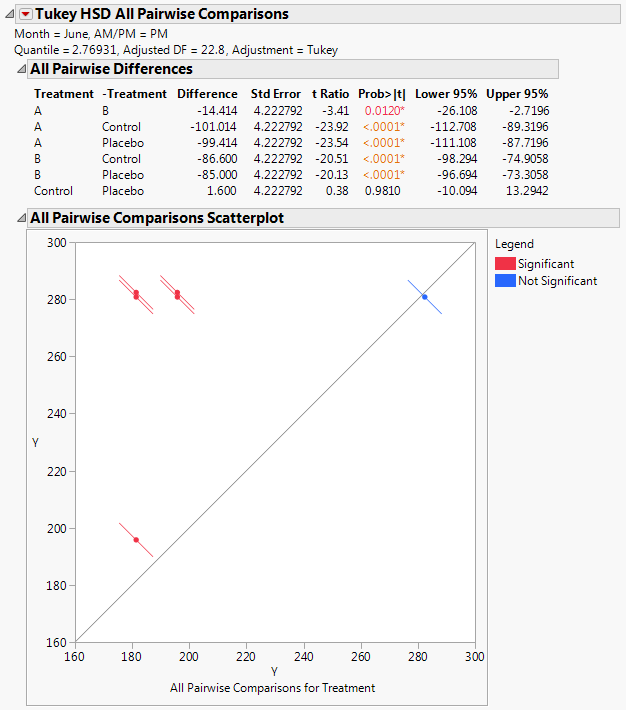
Click the red triangle next to Fit Mixed and select Multiple Comparisons.

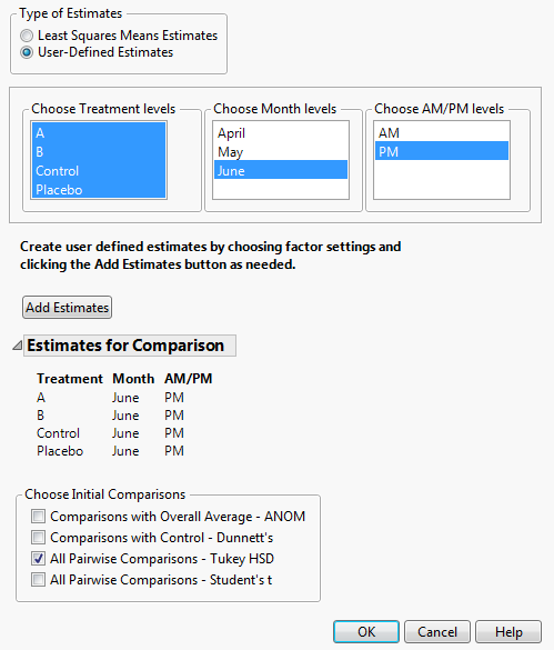
Under Types of Estimates, select User-Defined Estimates.

From the Choose Treatment levels panel, select all four treatment types.

From the Choose Month levels panel, select June.

From the Choose AM/PM levels panel, select PM.

Click Add Estimates.

From the Choose Initial Comparisons list, select All Pairwise Comparisons - Tukey HSD.

The Multiple Comparisons window should appear as shown in Completed Multiple Comparisons Window.

Completed Multiple Comparisons Window

Click OK.

Tukey HSD All Pairwise Comparisons Report for All Treatments for June PM

The Tukey HSD All Pairwise Comparisons report shows an All Pairwise Differences report and an All Pairwise Comparisons Scatterplot. All treatments other than the Control and Placebo differ significantly on the June PM measurements.

Consider the difference between treatments A and B. The difference in means is -14.414 and the confidence interval ranges from -26.108 to -2.7196. You conclude that the reduction in cholesterol measurements due to treatment A exceeds the reduction by treatment B by somewhere between 2.7 and 26.1 points. Both treatments A and B are highly effective compared to the Control and Placebo.

Conduct an Equivalence Test

Suppose that the scientist with whom you are working considers a change of no more than three points to be equivalent to no change from a practical perspective. Conduct an equivalence test to see whether the effect of AM/PM is of practical interest.

Select Multiple Comparisons from the Fit Mixed red triangle menu.

Select AM/PM from the Choose an Effect list.

Select All Pairwise Comparisons - Tukey HSD from the Choose Initial Comparisons list.

Click OK.

The report shows that the estimated difference between the afternoon and morning observations is 4.00261. Though this is statistically significant, is it sufficiently larger than the 3-point equivalence margin to be considered of practical interest?

Select Equivalence Tests from the Tukey HSD All Pairwise Comparisons red triangle menu.

Type 3 in the box for Difference considered practically zero.

Click OK.

The Equivalence TOST Tests report and Equivalence Test Scatterplot show that the -4.00261 point difference is not within the three-point margin. Therefore, the difference is of practical interest.

Equivalent TOST Test and Equivalence Test Scatterplot for AM/PM Effect

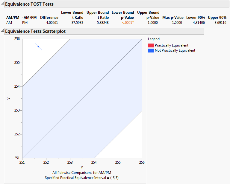
Note: The equivalence test consists of two one-sided t tests for the null hypotheses that the true difference is either below -3 or above 3. If both tests reject, this indicates that the difference in the means falls between -3 and 3, and the groups are considered practically equivalent.

Regression Model for AR(1) Model Example

Using the Month and AM/PM categorical effects, you have compared four covariance structures for the cholesterol data. (Note that a categorical effect was required for the Unstructured fit.) You have decided to use an AR(1) covariance structure.

Suppose now that you want to model the effect of treatment in terms of the continuous effect Days instead of the categorical effects. You can then predict cholesterol levels at arbitrary time during treatment.

After following step 1 to step 8.19 in Covariance Structure: Toeplitz, return to the Fit Model launch window.

On the Fixed Effects tab, select the existing fixed effects and click Remove.

Select Treatment and Days then select Macros > Full Factorial.

Fit Model Launch Window Showing Fixed Effects Tab

Click Run.

The Fit Mixed report is shown in Fit Mixed Report - AR(1) Covariance Structure with Continuous Fixed Effect. You see that the interaction of Treatment and Days is highly significant indicating different regressions for the drugs.

Note: To predict outcomes for the drugs at different days, use the profiler. See Profiler in the Profilers book for more information.

Fit Mixed Report - AR(1) Covariance Structure with Continuous Fixed Effect