Conduct Prospective Power Analysis for a Nonlinear Model

In this example, you are interested in the main effects of six continuous factors on whether a part passes or fails inspection. The response is binomial and you can afford a total of 60 runs.

You will do the following:

Construct a custom design for your experiment. See Construct the Design.

Note: Although a custom design is not optimal for a non-linear situation, in this example, for simplicity, you will use the Custom Design platform rather than the Nonlinear Design platform. For an example illustrating why a design constructed using the Nonlinear Design platform is better than an orthogonal design, see Examples of Nonlinear Designs in the Design of Experiments Guide.

Fit a logistic model using the Generalized Linear Model personality. See Fit the Generalized Linear Model.

Simulate likelihood ratio test p-values to explore the power of detecting a difference over a range of probability values that is determined by the linear predictor. See Explore Power.

Plan for the Example

You will model the probability of a success using a generalized linear model with the logit as a link function. The logit link function fits a logistic model:

where π(X) denotes the probability that a part passes at the given design settings X = (X1, X2, ..., X6).

Denote the linear predictor by L(X):

You will explore power for the following values of the coefficients of the linear predictor:

Coefficient	Value
β0	0
β1	1
β2	.9
β3	.8
β4	.7
β5	.6
β6	.5

Because the intercept in the linear predictor is 0, when all factors are set to 0, the probability of a passing part equals 50%. The probabilities associated with the levels of the ith factor, when all other factors are set to 0, are given below.

Factor	Percent Passing at Xi = 1	Percent Passing at Xi = -1	Difference
X1	73.11%	26.89%	46.2%
X2	71.09%	28.91%	42.2%
X3	69.00%	31.00%	38.0%
X4	66.82%	33.18%	33.6%
X5	64.56%	35.43%	29.1%
X6	62.25%	37.75%	24.5%

For example, when all factors other than X1 are set to 0, the difference in pass rates that you want to detect is 46.2%. The smallest difference in pass rates that you want to detect occurs when all factors other than X6 are set to zero and that difference is 24.5%.

Construct the Design

Note: If you prefer to skip the steps in this section, select Help > Sample Data Library and open Design Experiment/Binomial Experiment.jmp. Click the green triangle next to the DOE Simulate script and then go to Define Simulated Responses.

Select DOE > Custom Design.

In the Factors outline, type 6 next to Add N Factors.

Click Add Factor > Continuous.

Click Continue.

You are constructing a main effects design, so do not make any changes to the Model outline.

Under Number of Runs, type 60 next to User Specified.

Click the Custom Design red triangle and select Simulate Responses.

This opens the Simulate Responses window after you select Make Table to construct the design table.

Note: Setting the Random Seed in step 7 and Number of Starts in step 8 reproduces the same design shown in this example. In constructing a design on your own, these steps are not necessary.

(Optional) Click the Custom Design red triangle and select Set Random Seed. Type 12345 and click OK.

(Optional) Click the Custom Design red triangle and select Number of Starts. Type 1 and click OK.

Click Make Design.

10.

Click Make Table.

Note: The entries in your Y and Y Simulated columns will differ from those that appear in Figure 9.121.

Figure 9.121 Partial View of Design Table

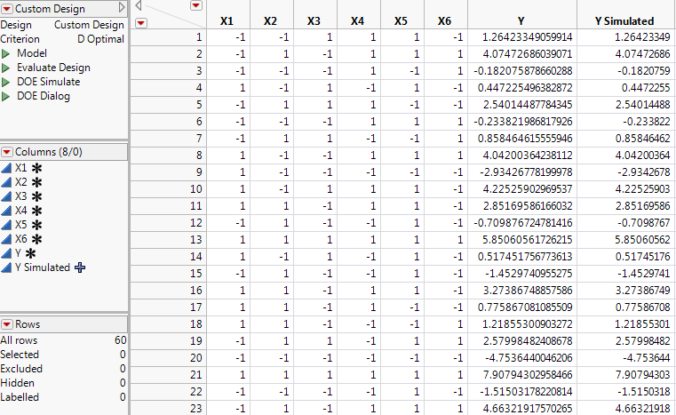
Figure 9.122 Simulate Responses Window

The design table and a Simulate Responses window appear. Two columns are added to the design table:

–

Y contains a set of values simulated according to the specifications in the Simulate Responses window.

–

Y Simulated contains a formula that calculates its values using the formula for the model that is specified in the Simulate Responses window. To view the formula, click on the plus sign to the right of the column name in the Columns panel.

Continue to the next section, where you simulate binomial responses and fit a generalized linear model to these simulated responses.

Define Simulated Responses

Your plan is to simulate binomial response data where the probability of success is given by a logistic model. For more information on Simulate Response, see Simulate Responses in the Design of Experiments Guide.

Note: If you prefer to skip the steps in this section, click the green triangle next to the Simulate Model Responses script. Then go to Fit the Generalized Linear Model.

In the Simulate Responses window (Figure 9.122), type the following values under Y:

–

Next to Intercept, type 0.

–

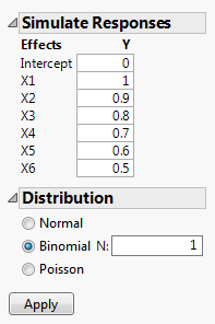
Next to X1, 1 is entered by default. Keep that value.

–

Next to X2, type 0.9.

–

Next to X3, type 0.8.

–

Next to X4, type 0.7.

–

Next to X5, type 0.6.

–

Next to X6, type 0.5.

In the Distribution outline, select Binomial.

Leave the value for N set to 1, indicating that there is only one unit per trial.

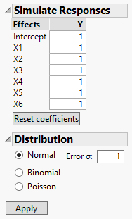
Figure 9.123 Completed Simulate Responses Window

Click Apply.

In the design data table, the Y Simulated column is replaced with a formula column that generates binomial values. A column called Y N Trials indicates the number of trials for each run.

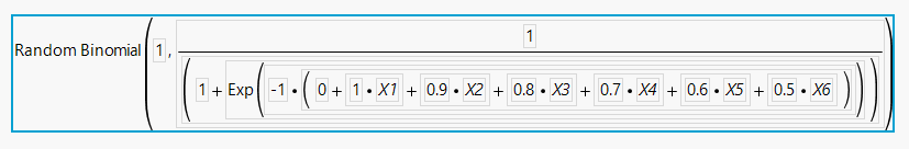
(Optional) Click on the plus sign to the right of Y Simulated in the Columns panel.

Figure 9.124 Random Binomial Formula for Y Simulated

Click Cancel.

Fit the Generalized Linear Model

In the data table, click the green triangle next to the Model script.

Click the Y variable next to the Y button and click Remove.

Click Y Simulated and click the Y button.

You are replacing Y with a column that contains randomly generated binomial values.

From the Personality menu, select Generalized Linear Model.

From the Distribution menu, select Binomial.

Notice that the Logit function appears in the Link Function menu.

Click Run.

The model that is fit is based on a single set of simulated binomial responses.

Explore Power

Next, explore the power of tests to detect a difference over the range of probability values determined by the linear predictor with the coefficient values given in Plan for the Example.

In the Effect Tests outline, right-click in the Prob>ChiSq column and select Simulate.

Figure 9.125 Simulate Window

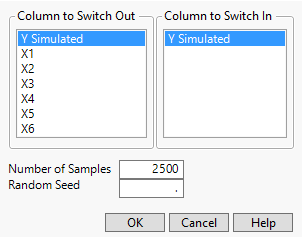
Make sure the Y Simulated column is selected in the Column to Switch Out list. This column contains the values that were used to fit the model. When you select the column Y Simulated under Column to Switch In, for each simulation, you are telling JMP to replace the values in Y Simulated with a new column of values that are simulated using the formula in the column Y Simulated.

The column you have selected in the report, Prob>ChiSq, is the p-value for a likelihood ratio test of whether the associated main effect is 0. The Prob>ChiSq value will be simulated for each effect listed in the Effect Tests table.

Next to Number of Samples, enter 500.

Click OK.

A Generalized Linear Model Simulate Results data table appears.

Note: Because response values are simulated, your simulated p-values will differ from those shown in Figure 9.126.

Figure 9.126 Table of Simulated Results, Partial View

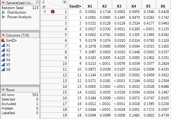
The first row of the table contains the initial values of Prob>ChiSq and is excluded. The remaining 500 rows contain simulated values.

Run the Power Analysis script.

Note: Because response values are simulated, your simulated power results will differ from those shown in Figure 9.127.

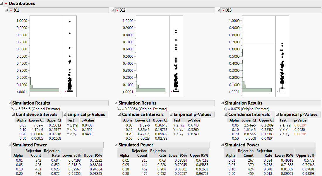
Figure 9.127 Distribution Plots for the First Three Effects

The histograms plot the 500 simulated Prob>ChiSq values for each main effect. The Simulated Power outline shows the simulated Rejection Rate in the 500 simulations.

For easier viewing, stack the reports and de-select the plots, as follows.

Click the Distributions red triangle and select Stack.

Press Ctrl and click the X1 red triangle, and de-select Outlier Box Plot.

Press Ctrl and click the X1 red triangle, then select Histogram Options and de-select Histogram.

Note: Because response values are simulated, your simulated power results will differ from those shown in Figure 9.128.

Figure 9.128 Power Results for the First Three Effects

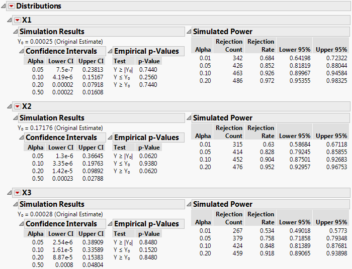
In the Simulated Power outlines, the Rejection Rate for each row gives the proportion of p-values that are smaller than the corresponding Alpha. For example, for X3, which corresponds to a coefficient value of 0.8 and a probability difference of 38%, the simulated power for a 0.05 significance level is 379/500 = 0.758. Table 9.5 summarizes the estimated power at the 0.05 significance level for all effects. Notice how power decreases as the Difference to Detect decreases. Also notice that the power to detect an effect as large as 24.5% (X6) is only approximately 0.37.

Note: Because response values are simulated, your simulated power results will differ from those shown in Table 9.5.

Table 9.5 Simulated Power at Significance Level 0.05
Factor	Percent Passing at Xi = 1	Percent Passing at Xi = -1	Difference to Detect	Simulated Power (Rejection Rate) at Alpha=0.05
X1	73.11%	26.89%	46.2%	0.852
X2	71.09%	28.91%	42.2%	0.828
X3	69.00%	31.00%	38.0%	0.758
X4	66.82%	33.18%	33.6%	0.654
X5	64.56%	35.43%	29.1%	0.488
X6	62.25%	37.75%	24.5%	0.372