Inverse Prediction

Inverse prediction occurs when you use a statistical model to infer the value of an explanatory variable, given a value of the response variable. Inverse prediction is sometimes referred to as calibration.

By selecting Inverse Prediction on the Estimates menu, you can estimate values of an independent variable, X, that correspond to specified values of the response (Figure 3.37). In addition, you can specify values for other explanatory variables in the model (Figure 3.37). The inverse prediction computation provides confidence limits for values of X that correspond to the specified response value. You can specify the response value to be the mean response or simply an individual response. For an example, see Example of Inverse Prediction.

Analyzing Multiple Explanatory Variables

When the model includes multiple explanatory variables, you can predict the value of X for the specified values of the other variables. You might want to predict the amount of running time that results in an oxygen uptake of 50 when one’s resting pulse rate is 60. You might want separate inverse predictions for both males and females. Specify these requirements using the inverse prediction option.

The inverse prediction window shows the list of explanatory variables to the left. (See Figure 3.37 for an example.) Each continuous variable is initially set to its mean. Each nominal or ordinal variable is set to its lowest level (in terms of value ordering). You must remove the value for the variable that you want to predict, setting it to missing. Also, you must specify the values of the other variables for which you want your inverse prediction to hold (if these differ from the default settings). In the list to the right in the window, you can supply one or more response values of interest. For an example, see Example of Predicting a Single X Value with Multiple Model Effects.

Note: The confidence limits for inverse prediction can sometimes result in a one-sided or even an infinite interval. For technical details, see Inverse Prediction with Confidence Limits in Statistical Details.

Example of Inverse Prediction

In this example, you fit a regression model that predicts oxygen uptake from Runtime. Then you estimate the Runtime values that result in specified oxygen uptake values. There is only a single X, Runtime, so you start by using the Fit Y by X platform to obtain a visual approximation of the inverse prediction values.

Select Help > Sample Data Library and open Fitness.jmp.

Select Analyze > Fit Y by X.

Select Oxy and click Y, Response.

Select Runtime and click X, Factor.

Click OK.

From the red triangle menu, select Fit Line.

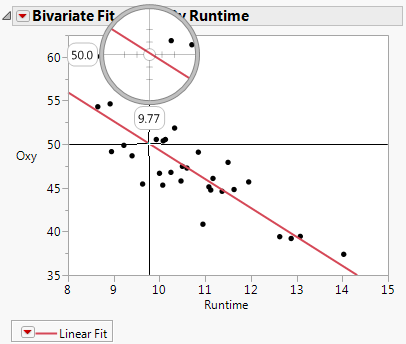
Use the crosshair tool as described below to approximate the Runtime value that results in a mean Oxy value of 50.

Select Tools > Crosshairs.

Click the Oxy axis at about 50 and then drag the cursor so that the crosshairs intersect with the prediction line.

Figure 3.34 shows that a Runtime of about 9.77 gives an inverse prediction of about 50 for Oxy.

Figure 3.34 Bivariate Fit for Fitness.jmp

To obtain an exact prediction for Runtime, along with a confidence interval, use the Fit Model launch window as follows:

From the Fitness.jmp sample data table, select Analyze > Fit Model.

Select Oxy and click Y.

Select Runtime and then click Add.

Click Run.

From the red triangle menu next to Response Oxy, select Estimates > Inverse Prediction.

Enter four values for Oxy as shown in Figure 3.35.

Click OK.

Figure 3.35 Completed Inverse Prediction Specification Window

The Inverse Prediction report (Figure 3.36) gives predicted Runtime values that correspond to each specified Oxy value. The report also shows upper and lower 95% confidence limits for these Runtime values, relative to obtaining the mean response.

Figure 3.36 Inverse Prediction Report

The exact predicted Runtime resulting in an Oxy value of 50 is 9.7935. This value is close to the approximate Runtime value of 9.77 found in the Bivariate Fit report shown in Figure 3.34. The Inverse Prediction report also gives a plot showing the linear relationship between Oxy and Runtime and the confidence intervals.

Example of Predicting a Single X Value with Multiple Model Effects

This example predicts the Runtime that results in oxygen uptake of 50 when RstPulse is 60. The Runtime is predicted for both males and females.

From the Fitness.jmp sample data table, select Analyze > Fit Model.

Select Oxy and click Y.

Select Sex, Runtime, and RstPulse and then select Add.

Click Run.

From the red triangle menu next to Response Oxy, select Estimates > Inverse Prediction.

Delete the value for Runtime, because you want to predict that value.

Select the All box next to Sex to estimate Runtime for all levels of Sex.

Replace the mean for RstPulse with 60.

Enter the value 50 for Oxy as shown in Figure 3.37.

10.

Click OK.

Figure 3.37 Inverse Prediction Specification for a Multiple Regression Model

The report, shown in Figure 3.38, gives the predicted values of Runtime for both females and males. The report also includes 95% confidence intervals for Runtime values that give a mean response of 50.

Figure 3.38 Inverse Prediction Report for a Multiple Regression Model

The plot shows the linear fits for females and males, given that RstPulse is 60. The two confidence intervals are shown in red and blue, respectively. Note that the intervals overlap, indicating that the true values of Runtime leading to an Oxy value of 50 might be identical for both males and females.