Leverage Plot Details

Effect leverage plots are also referred to as partial-regression residual leverage plots (Belsley et al. 1980) or added variable plots (Cook and Weisberg 1982). Sall (1990) generalized these plots to apply to any linear hypothesis.

JMP provides two types of leverage plots:

•

Effect Leverage plots show observations relative to the hypothesis that the effect is not in the model, given that all other effects are in the model.

•

The Whole Model leverage plot, given in the Actual by Predicted Plot report, shows the observations relative to the hypothesis of no factor effects.

In the Effect leverage plot, only one effect is hypothesized to be zero. However, in the Whole Model Actual by Predicted plot, all effects are hypothesized to be zero. Sall (1990) generalizes the idea of a leverage plot to arbitrary linear hypotheses, of which the Whole Model leverage plot is an example. The details from that paper, summarized in this section, specialize to the two types of plots found in JMP.

Construction

Suppose that the estimable hypothesis of interest is

The leverage plot characterizes this test by plotting points so that the distance of each point to the sloped regression line displays the unconstrained residual. The distance to the horizontal line at 0 displays the residual when the fit is constrained by the hypothesis. The difference between the sums of squares of these two sets of residuals is the sum of squares due to the hypothesis. This value becomes the main component of the F test.

The parameter estimates constrained by the hypothesis can be written

Here b is the least squares estimate

and lambda is the Lagrangian multiplier for the hypothesis constraint, calculated by

The unconstrained and hypothesis-constrained residuals are, respectively,

For each observation, consider the point with horizontal axis value vx and vertical axis value vy where:

•

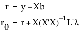
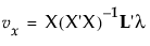
vx is the constrained residual minus the unconstrained residual, r0 - r, reflecting information left over once the constraint is applied

•

vy is the horizontal axis value plus the unconstrained residual

Thus, these points have x and y coordinates

and

These points form the basis for the leverage plot. This construction is illustrated in Figure 3.68, where the response mean is 0 and slope of the solid line is 1.

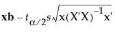
Leverage plots in JMP have a dotted horizontal line at the mean of the response,

. The plotted points are given by (vx +

, vy).

Figure 3.68 Construction of Leverage Plot

Superimposing a Test on the Leverage Plot

In simple linear regression, you can plot the confidence limits for the expected value of the response as a smooth function of the predictor variable x

Upper (x) =

Lower (x) =

where x = [1 x] is the 2-vector of predictors.

These confidence curves give a visual assessment of the significance of the corresponding hypothesis test, illustrated in Figure 3.57:

•

Significant: If the slope parameter is significantly different from zero, the confidence curves cross the horizontal line at the response mean.

•

Borderline: If the t test for the slope parameter is sitting right on the margin of significance, the confidence curve is asymptotic to the horizontal line at the response mean.

•

Not Significant: If the slope parameter is not significantly different from zero, the confidence curve does not cross the horizontal line at the response mean.

Leverage plots mirror this thinking by displaying confidence curves. These are adjusted so that the plots are suitably centered. Denote a point on the horizontal axis by z. Define the functions

Upper(z) =

and

Lower(z) =

where F is the F statistic for the hypothesis and

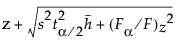
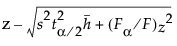
is the reference value for significance level α.

And

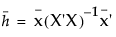, where

is a row vector consisting of suitable middle values for the predictors, such as their means.

These functions behave in the same fashion as do the confidence curves for simple linear regression:

•

If the F statistic is greater than the reference value, the confidence functions cross the horizontal axis.

•

If the F statistic is equal to the reference value, the confidence functions have the horizontal axis as an asymptote.

•

If the F statistic is less than the reference value, the confidence functions do not cross.

Also, it is important that Upper(z) - Lower(z) is a valid confidence interval for the predicted value at z.