Multiple Responses with Five Mixture Variables

This example uses the Five Factor Mixture.jmp sample data table. There are five components (x1 to x5), one categorical process factor (Type), and three responses, Y1, Y2, and Y3. A response surface model is fit to each response and the prediction equations are saved in Y1 Predicted, Y2 Predicted, and Y3 Predicted.

Select Help > Sample Data Library and open Five Factor Mixture.jmp.

Select Graph > Mixture Profiler.

Select Y1 Predicted, Y2 Predicted, and Y3 Predicted and click Y, Predicted.

Click OK.

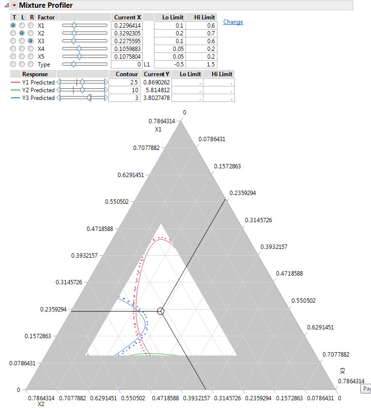
Enter 3 in the Contour edit box for Y3 Predicted so that the contour is visible on the plot.

Figure 6.11 Mixture Profiler with Y3 Predicted Contour Set to 3

A few items to note about the output in Figure 6.11.

•

The on axis factors are X1, X2, and X3 as indicated by the axes labels and the radio buttons in the factor settings. All of the factors have low and high limits, which were entered previously as Column Properties. See Column Properties in the Using JMP book for more information about entering column properties. Alternatively, you can enter the low and high limits directly by entering them in the Lo Limit and Hi Limit boxes.

•

The white unshaded region is the feasible region. This is determined by the factor limits.

•

The on-axis factors, x1, x2, and x3, radio buttons are selected.

•

The categorical factor, Type, has a radio button, but it cannot be assigned to the plot. The current value for Type is L1, which is listed immediately to the right of the Current X box. The Current X box for Type uses a 0 to represent L1.

•

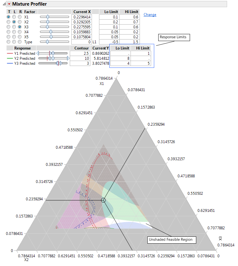
All three prediction equations have contours on the plot and are differentiated by color.

Suppose the manufacturer desires to hold Y1 less than 1, Y2 greater than 8 and Y3 between 4 and 5, with a target of 4.5. The Mixture Profiler can help you investigate the response surface and find optimal factor settings.

Enter1 in the Y1 Predicted Hi Limit edit box. Enter 8 in the Y2 Predicted Lo Limit edit box. Enter 4 in theY3 Predicted Lo Limit edit box and 5 in the Y3 Predicted Hi Limit edit box.

The feasible region remains white (unshaded). Use the Response slider controls to position the contours in the feasible region. Alternatively, move the cross hair into the feasible region

Figure 6.12 Feasible Region After Setting Response Limits

Select the magnifier tool

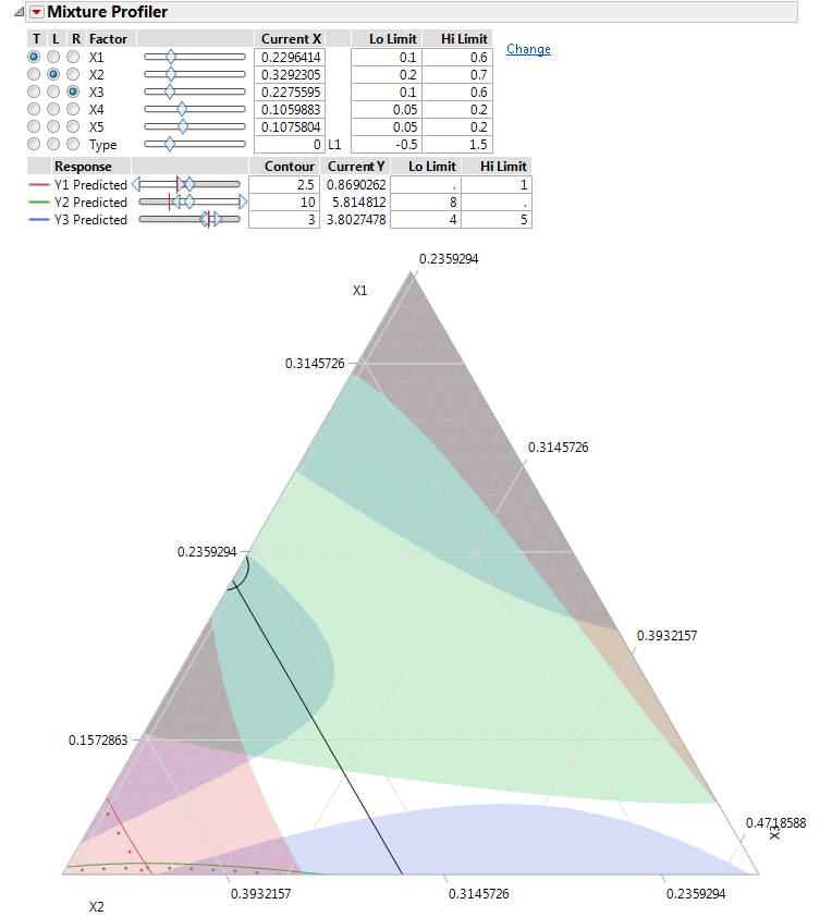
to zoom in on the feasible region.

Figure 6.13 Ternary Plot with Enlarged Feasible Region

The manufacturer wants to maximize Y1, minimize Y2, and have Y3 at 4.5.

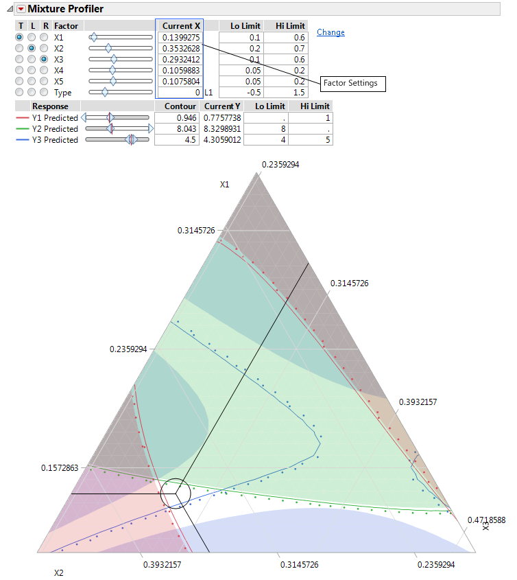
Use the slider controls or Contour edit boxes for Y1 Predicted to maximize the red contour within the feasible region. The Up Dots show direction of increasing predicted response.

10.

Use the slider controls or Contour edit boxes for Y2 Predicted to minimize the green contour within the unshaded region.

11.

Enter 4.5 in the Contour edit box for Y3 Predicted to set the blue contour to the target value.

The resulting three contours do not all intersect at one spot. Y1 and Y2 cannot be optimized with Y3 on target, so you have to compromise. Position the three-way crosshairs in the middle of the contours to explore the factor levels that produce those response values. Note that these response contours are for the current settings of x4, x5, and Type.

Figure 6.14 Factor Settings for Optimal Results

12.

Click the Mixture Profiler red triangle and select Factor Settings > Remember Settings to save the current settings. The settings are appended to the bottom of the report window.

Figure 6.15 Remembered Settings

With the current settings saved, you can now change the values of x4, x5 and Type to explore their impact on the feasible region. You can compare the factor settings and response values for each level of Type by referring to the Remembered Settings report.