The Custom Design platform facilitates the task of data analysis by saving a Model script to the design table that it creates. See Figure 2.10. Run this script after you conduct your experiment and enter your data. The script opens a Fit Model window containing the effects that you specified in the Model outline of the Custom Design window.
|
1.
|
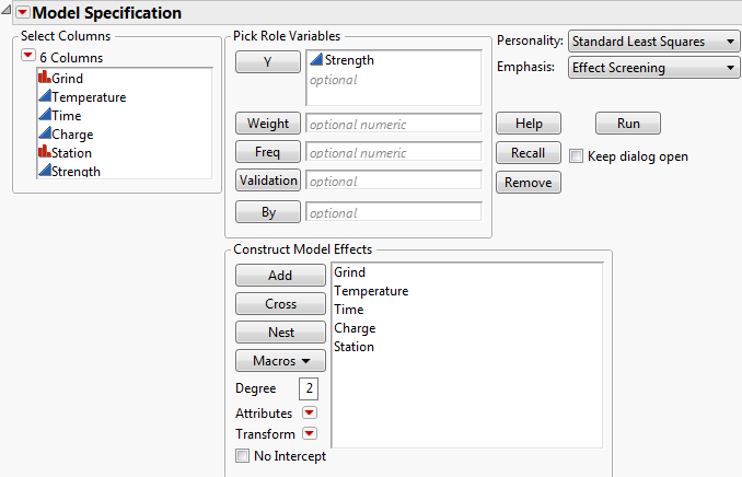
Figure 2.12 Model Specification Window
|
3.
|
Select the Keep dialog open option.
|
|
4.
|
Click Run.
|
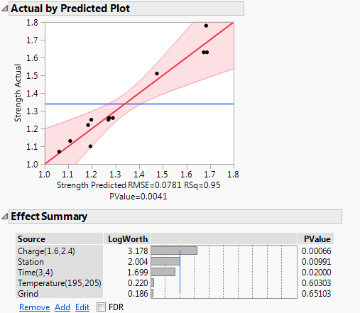
The Effect Summary and Actual by Predicted Plot reports give high-level information about the model.
|
•
|
The model is significant, as indicated by the Actual by Predicted Plot. The notation P = 0.0041, shown below the plot, gives the significance level of the overall model test.
|
|
•
|
|
•
|
Because Temperature and Grind appear not to be active, they contribute random noise to the model. Refit the model without these effects to obtain more precise estimates of the model parameters associated with the active effects.
|
1.
|
In the Model Specification window, select Temperature and Grind in the Construct Model Effects list.
|
|
2.
|
Click Remove.
|
|
3.
|
|
4.
|
Click Run.
|
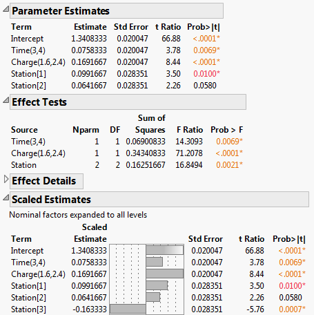
Figure 2.14 Partial Output for the Reduced Model
|
•
|
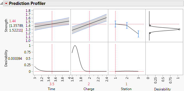
Figure 2.15 Prediction Profiler
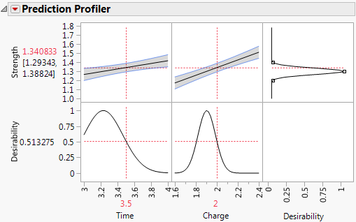
Recall that, in designing your experiment, you set a response Goal of Match Target with limits of 1.2 and 1.4. JMP uses this information to construct a desirability function to reflect your specifications. For more details, see Factors.
|
•
|
The first two plots in the top row of the graph show how Strength varies for one of the factors, given the setting of the other factor. For example, when Charge is 2, the line in the plot for Time shows how predicted Strength changes with Time.
|
|
•
|
The values to the left of the top row of plots give the Predicted Strength (in red) and a confidence interval for the mean Strength for the selected factor settings.
|
|
•
|
The right-most plot in the top row shows the desirability function for Strength. The desirability function indicates that the target of 1.3 is most desirable. Desirability decreases as you move away from that target. Desirability is close to 0 at the limits of 1.2 and 1.4.
|
Explore various factor settings by dragging the red dashed vertical lines in the columns for Time and Charge. Since there are no interactions in the model, the profiler indicates that increasing Charge increases Strength. Also, Strength seems to be more sensitive to changes in Charge than to changes in Time.
Since Station is a blocking factor, it does not appear in the Prediction Profiler. However, you might like to see how predicted Strength varies by Station. To include Station in the Prediction Profiler, follow these steps:
|
1.
|
From the Prediction Profiler red triangle menu, select Reset Factor Grid.
|
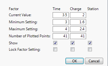
A Factor Settings window appears with columns for Time, Charge, and Station. Under Station, notice that the box corresponding to Show is not selected. This indicates that Station is not shown in the Prediction Profiler.
|
2.
|
|
3.
|
Figure 2.16 Factor Settings Window
|
4.
|
Click OK.
|
Plots for Station appear in the Prediction Profiler.
|
5.
|
Click in either plot above Station to insert a dashed red vertical line.
|
|
6.
|
Move the dashed red vertical line to Station 1.
|
|
7.
|
Move the dashed red vertical line to Station 3.
|
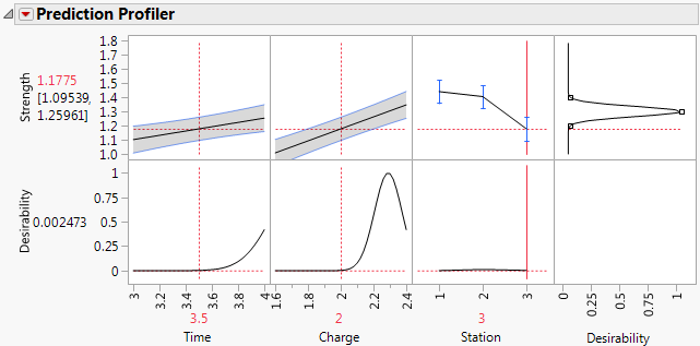
The predicted Strength in the center of the design region for Station 1 is 1.44. For Station 3, the predicted Strength is about 1.18. The magnitude of the difference indicates that you need to address Station variability. Better control of Station variation should lead to more consistent Strength. Once Station consistency is achieved, you can determine common optimal settings for Time and Charge.