This example shows how to create a nonlinear design when you have prior data. In this example, the data pertain to a chemical reaction. You want to model the rate of uptake (velocity) of available organic substrate as a function of the concentration of that substrate. See Meyers (1986). You have already run an experiment, but you want to leverage your results to obtain more precise estimates of the parameters.
|
1.
|
|
2.
|
Click the plus sign next to Model (x) in the Columns panel. The formula editor opens.
|
|
3.
|
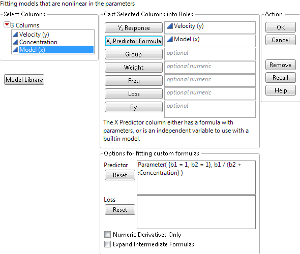
TheParameters outline in the middle bottom of the formula editor shows the current values of the model parameters.The values (b1 = 1 and b2 = 1) are your initial estimates. They are used to compute the Model (x) values in the data table. For your next experiment, you want to replace these with better estimates.
|
|
4.
|
Click Cancel to close the formula editor window.
|
|
5.
|
Select Analyze > Specialized Modeling > Nonlinear.
|
|
6.
|
|
7.
|
Notice that the formula given by Model (x) appears in the Options for fitting custom formulas panel.
Figure 22.7 Nonlinear Analysis Launch Window
|
8.
|
Click OK.
|
|
9.
|
|
10.
|
In the Control Panel, click Confidence Limits.
|
Figure 22.8 Nonlinear Fit Results
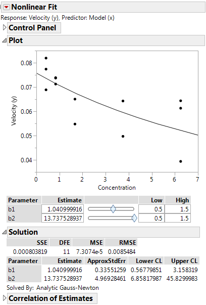
The Lower CL and Upper CL values for b1 and b2 define ranges of values for these parameters. Next, use these intervals to define a range for the prior values in your augmented nonlinear design.
|
1.
|
|
2.
|
|
3.
|
|
4.
|
Click OK.
|
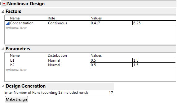
In the Chemical Kinetics.jmp data, the values for Concentration range from 0.417 to 6.25. Therefore, these values initially appear as the low and high values in the Factors outline. You want to change these values to encompass a broader interval.
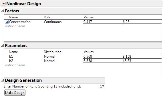
The range of Values for the parameters reflects the uncertainty of your knowledge about them. You could specify a range that you think covers 95% of possible parameter values. The confidence limits from the Nonlinear Fit report shown in Figure 22.8 provide such a range. Replace the Values for the parameters in the Parameters outline with the confidence limits, rounding to three decimal places.
|
–
|
b1: 0.568 and 3.158
|
|
–
|
bb2: 6.858 and 45.830
|
Figure 22.10 Updated Values for Factor and Parameters
|
8.
|
Enter 40 for the Number of Runs in the Design Generation panel.
|
|
9.
|
Click Make Design.
|
The Design outline opens, showing the Concentration and Velocity (y) values for the original 13 runs and new Concentration settings for the additional 27 runs.
|
10.
|
Click Make Table.
|
The new runs reflect the broader interval of Concentration values and the range of values for b1 and b2 obtained from the original experiment, which are used to define the prior distribution. Both should lead to more precise estimates of b1 and b2.