Create a Design for a Binomial Response

In some applications, the measurement of interest is a pass/fail (binomial) measurement. In this example, you will construct a nonlinear design for a binomial response with one design factor. For more information on designs in nonlinear settings and the binomial case in particular, see Gotwalt (2009).

You plan to model the probability of success for your binomial response as a function of a single factor x. using a generalized linear model with a logistic link function

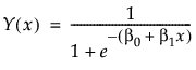
and the variance of Y as the weight.

This model is nonlinear in the unknown parameters β0, and β1. Use the nonlinear designer to plan an experimental design.Your goal is to model the effect of x on your binomial response Y.

To generated the desired non-linear design you must have a data table containing columns for the predictor, a column containing a formula for the nonlinear response model that you are fitting, and a column with a formula for your weights.

Data Table for Design Construction

The One Factor Logistic Design.jmp data table, found in the Design Experiment folder, contains the following:

•

Column x for the predictor. The Coding property defined for this column sets the low value to 0 and the high value to 1.

•

Column Y, for the response. This is the column for collected responses (0/1) from your testing.

•

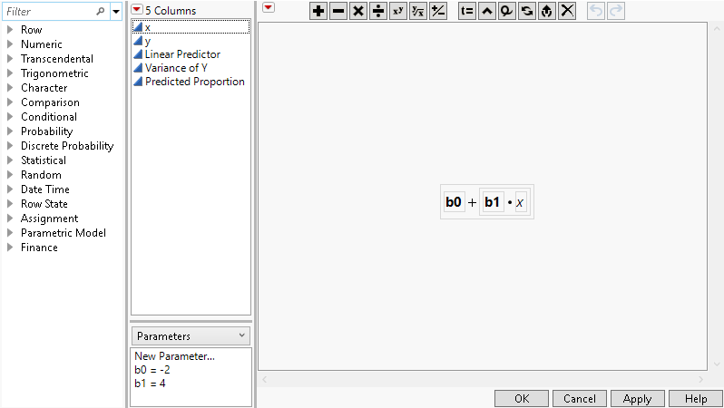
Column Linear Predictor that contains a formula for the linear portion of the link function. To view the formula, click on the plus sign to the right of Linear Predictor in the Columns panel. The model formula includes the initial estimates for the parameters b0 and b1. Initial parameter values are set when you define a formula. These values are shown in the formula element panel in the lower center of the formula editor window.

Figure 22.11 Linear Predictor Formula with Initial Parameter Estimates

•

Column Variance of Y that contains the formula for the variance of the response based on the assumed logistic model. This is p(1-p) where p is the logistic function. This column is used as the weight column.

•

Column Predicted Proportion that contains the logistic link function.

Create the Design

Select Help > Sample Data Library and open Design Experiment/One Factor Logistic Design.jmp.

Select DOE > Special Purpose > Nonlinear Design.

Select Y and click Y, Response.

Select Linear Predictor and click X, Linear Predictor .

Select Variance of Y and click Weight.

Click OK.

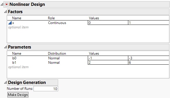
Figure 22.12 Nonlinear Design Window

The Factors outline shows the factor x with the specified values of 0 and 1. The Parameters outline shows the two model parameters with each prior distribution set to a normal distribution. JMP computes default Values based on your initial settings for the parameter values. You can change the assumed distribution and ranges for the parameters in this outline. Leave all settings as they appear. The default number of runs is 10.

Click the Nonlinear Design red triangle and select Advanced Options > N Monte Carlo Spheres. Set the number of spheres to 0 to obtain a locally optimal design. Click OK.

Click Make Design.

Click Augment Table.

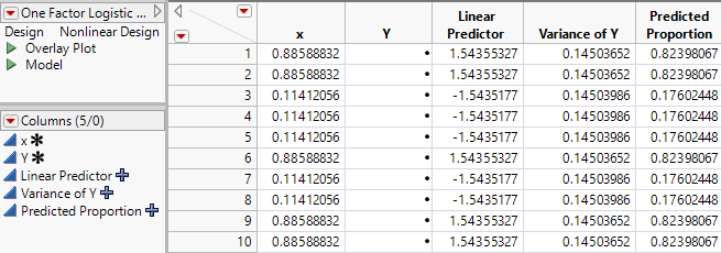
This adds the 10 run design to One Factor Logistic Design.jmp, see Figure 22.13. Your design table will be different because the optimization algorithm has a random component.

Figure 22.13 Augmentation of Binomial Optimal Start.jmp

The model saved to the data table is a nonlinear model to fit the “Linear Predictor” used in the creation of the design. To model the effect of x on Y use a generalized linear model (GLM) with a logit link function. Simulate values for Y to explore the use of a GLM to evaluate your design.

Simulate Responses and Analyze

Right click on the Y column heading and select formula.

From the Random function list select Random Binomial.

Enter 1 for n and Predicted Proportion for p. Click OK

Select Analyze > Fit Model

Select Y and click Y.

Select x and click Add.

Select Generalized Linear Model as the personality.

Select Binomial as the Distribution.

Select Logit as the Link Function.

10.

Check Firth Bias-Adjusted Estimates.

11.

Click Run.

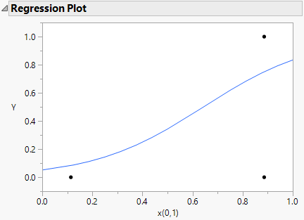
Figure 22.14 Regression Plot for Binomial DOE