Custom Test Option

Set up custom tests of effect levels using the Custom Test option.

Note: For instructions on how to create custom tests, see Custom Test in Standard Least Squares Report and Options.

The menu icon beside each effect name gives you the following options to request additional information about the multivariate fit:

Test Details

Displays the eigenvalues and eigenvectors of the

matrix used to construct multivariate test statistics. See Test Details.

Centroid Plot

Plots the centroids (multivariate least squares means) on the first two canonical variables formed from the test space. See Centroid Plot.

Save Canonical Scores

Saves variables called Canon[1], Canon[2], and so on, as columns in the current data table. These columns have both the values and their formulas. For an example, see Save Canonical Scores. For technical details, see Canonical Details.

Contrast

Performs the statistical contrasts of treatment levels that you specify in the contrasts dialog.

Note: The Contrast command is the same as for regression with a single response. See the LSMeans Contrast in Standard Least Squares Report and Options, for a description and examples of the LSMeans Contrast commands.

Test Details

The Test Details report gives canonical details about the test for the whole model or the specified effect.

Eigenvalue

The eigenvalues of the

matrix used in computing the multivariate test statistics.

Canonical Corr

The canonical correlations associated with each eigenvalue. This is the canonical correlation of the transformed responses with the effects, corrected for all other effects in the model.

Eigvec

The eigenvectors of the

matrix, or equivalently of

Example of Test Details

Select Help > Sample Data Library and open Iris.jmp.

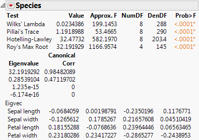
The Iris data (Mardia et al. 1979) have three levels of Species named Virginica, Setosa, and Versicolor. There are four measures (Petal length, Petal width, Sepal length, and Sepal width) taken on each sample.

Select Analyze > Fit Model.

Select Petal length, Petal width, Sepal length, and Sepal width and click Y.

Select Species and click Add.

For Personality, select Manova.

Click Run.

Click on the Choose Response button and select Identity.

Click Run.

From the red triangle menu next to Species, select Test Details.

The eigenvalues, eigenvectors, and canonical correlations appear. See Figure 8.4.

Figure 8.4 Test Details

Centroid Plot

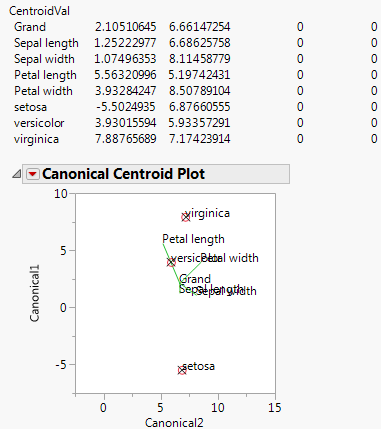
The Centroid Plot command (accessed from the red triangle next to Species) plots the centroids (multivariate least squares means) on the first two canonical variables formed from the test space, as in Figure 8.5. The first canonical axis is the vertical axis so that if the test space is only one dimensional the centroids align on a vertical axis. The centroid points appear with a circle corresponding to the 95% confidence region (Mardia et al. 1979). When centroid plots are created under effect tests, circles corresponding to the effect being tested appear in red. Other circles appear blue. Biplot rays show the directions of the original response variables in the test space. See Details for Centroid Plot Option.

Click the Centroid Val disclosure icon to show additional information, shown in Figure 8.5.

The first canonical axis with an eigenvalue accounts for much more separation than does the second axis. The means are well separated (discriminated), with the first group farther apart than the other two. The first canonical variable seems to load the petal length variables against the petal width variables. Relationships among groups of variables can be verified with Biplot Rays and the associated eigenvectors.

Figure 8.5 Centroid Plot and Centroid Values

Save Canonical Scores

Saves columns called Canon[i] to the data table, where i refers to the ith canonical score for the Y variables. The canonical scores are computed based on the

matrix used to construct the multivariate test statistic. Canonical scores are saved for eigenvectors corresponding to nonzero eigenvalues.

Canonical Correlation

Canonical correlation analysis is not a specific command, but it can be done by a sequence of commands in the multivariate fitting platform, as follows:

Follow step 1 through step 8 in Example of Test Details.

From the red triangle menu next to Whole Model, select Test Details.

From the red triangle menu next to Whole Model, select Save Canonical Scores.

The details list the canonical correlations (Canonical Corr) next to the eigenvalues. The saved variables are called Canon[1], Canon[2], and so on. These columns contain both the values and their formulas.

To obtain the canonical variables for the X side, repeat the same steps, but interchange the X and Y variables. If you already have the columns Canon[n] appended to the data table, the new columns are called Canon[n] 2 (or another number) that makes the name unique.

For another example, proceed as follows:

Select Help > Sample Data Library and open Exercise.jmp.

Select Analyze > Fit Model.

Select chins, situps, and jumps and click Y.

Select weight, waist, and pulse and click Add.

For Personality, select Manova.

Click Run.

Click on the Choose Response button and select Identity.

Click Run.

From the red triangle menu next to Whole Model, select Test Details.

10.

From the red triangle menu next to Whole Model, select Save Canonical Scores.

Figure 8.6 Canonical Correlations

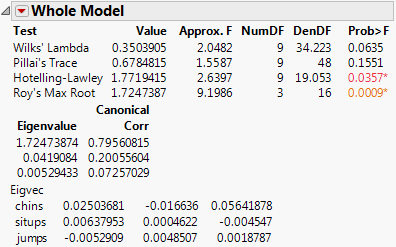
The output canonical variables use the eigenvectors shown as the linear combination of the Y variables. For example, the formula for Canon[1] is as follows:

0.02503681*chins + 0.00637953*situps + -0.0052909*jumps

This canonical analysis does not produce a standardized variable with mean 0 and standard deviation 1, but it is easy to define a new standardized variable with the calculator that has these features.