The Eigen() function performs eigenvalue decomposition of a symmetric matrix. Eigenvalue decompositions are used in many statistical techniques, most notably in principal components and canonical correlation, where the transformation associated with the largest eigenvalues are transformations that maximize variances.
Eigen() returns a list of matrices. The first matrix in the returned list is a column vector of eigenvalues; the second matrix contains eigenvectors as the columns.
A = [ 5 4 1 1, 4 5 1 1, 1 1 4 2, 1 1 2 4];
Eigen( A );
{[10, 5, 2, 1][0.632455532033676 - 0.316227766016838 - 2.77555756156289e-16 -0.707106781186547, 0.632455532033676 - 0.316227766016837 - 1.66533453693773e-16 0.707106781186547, 0.316227766016838 0.632455532033676 0.707106781186548 0, 0.316227766016837 0.632455532033676 - 0.707106781186547 0]}
{evals, evecs} = Eigen( A );
For some n × n matrix A, eigenvalue decomposition finds all λ (lambda) and vectors x, so that the equation Ax = λx has a nonzero solution x. The λ’s are called eigenvalues, and the corresponding x vectors are called eigenvectors. This is equivalent to solving (A - λI)x = 0. You can reconstruct A from eigenvalues and eigenvectors by a statement like the following:
newA = evecs * Diag( evals ) * evecs`;
[5.00000000000001 4 1 1,
4 5 1 1,
1 1 4 2,
1 1 2 4]
 .
.|
•
|
|
•
|
A * x = E` * Diag( M ) * E * x;
The Cholesky() function performs Cholesky decomposition. A positive semi-definite matrix A is re-expressed as the product of a nonsingular, lower-triangular matrix L and its transpose: L*L' = A.
E = [ 5 4 1 1, 4 5 1 1, 1 1 4 2, 1 1 2 4];
L = Cholesky( E );
[2.23606797749979 0 0 0,
1.788854381999832 1.341640786499874 0 0,
0.447213595499958 0.149071198499986 1.9436506316151 0,
0.447213595499958 0.149071198499986 0.914659120760047 1.71498585142509]
L*L`;
[5 4 1 1,
4 5 1 1,
1 1 4 2,
1 1 2 4]
Cholesky() is useful for reconstituting expressions into a more manageable form. For example, eigenvalues are available only for symmetric matrices in JMP, so the eigenvalues of the product AB could not be obtained directly. (Although A and B can be symmetric, the product is not symmetric.) However, you can usually rephrase the problem in terms of eigenvalues of L’BL where L is the Cholesky root of A, which has the same eigenvalues.
Another use of Cholesky() is in reordering matrices within Trace() expressions. Expressions such as Trace(A*B*A`) might involve huge operations counts if A has many rows. However, if B is small and can be factored into LL’ by Cholesky, then it can be reformulated to Trace(A*L*L`*A`). The resulting matrix is equal to Trace(L`A`*AL). This expression involves a much smaller number of operations, because it consists of only the sum of squares of the AL elements.
Use the function Chol Update() to update a Cholesky decomposition. If L is the Cholesky root of a n × n matrix A, then after using cholUpdate(L, C, V), L will be replaced with the Cholesky root of A+V*C*V'. C is an m × m symmetric matrix and V is an n × m matrix.
exS = [16 1 0 11 -1 12, 1 11 -1 1 -1 1, 0 -1 12 -1 1 0, 11 1 -1 11 -1 9, -1 -1 1 -1 9 -1, 12 1 0 9 -1 12];
exAchol = Cholesky( exS ); // conducts the Cholesky decomposition
exV = [1 1, 0 0, 0 1, 0 0, 0 0, 0 1];
// adds two column vectors to the design matrix
exC = [1 0, 0 -1];
/* The first column vector is added to one of the rows in the design matrix.
The second column vector is subtracted from one of the rows in the design matrix. */
exAnew = exS + exV * exC * exV`;
exAcholnew = Cholesky( exAnew );
// updates the Cholesky decomposition manually
Instead of manual updating, use Chol Update() to update the Cholesky decomposition, as follows:
exAcholnew_test = Chol Update( exAchol, exV, exC );
// updates the Cholesky decomposition more efficiently
Show( exAcholnew_test );
exAcholnew_test =
[ 4 0 0 0 0 0,
0.25 3.30718913883074 0 0 0 0, ...]
// results are the same as the manual process
Show( exAcholnew );
exAcholnew=
[ 4 0 0 0 0 0,
0.25 3.30718913883074 0 0 0 0, ...]
The SVD() function finds the singular value decomposition of a matrix. That is, for a matrix A, SVD() returns a list of three matrices U, M, and V, so that U*diag(M)*V`=A.
|
•
|
|
•
|
Singular value decomposition re-expresses A in the form USV’, where:
|
|
–
|
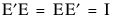
U and V are matrices that contain orthogonal column vectors (perpendicular, statistically independent vectors)
|
|
–
|
S is a n × n diagonal matrix containing the nonnegative square roots of the eigenvalues of A’A, the singular values of A.
|
A = [1 2 1 0, 2 3 0 1, 1 0 1 5, 0 1 5 1];
{U, M, V} = SVD( A );
newA = U * Diag( M ) * V`;
[1 2 0.999999999999997 -2.99456640040496e-15,
2 3 -1.17505831453979e-15 1,
0.999999999999997 -2.16851276518826e-15 0.999999999999999 5,
2.22586706011274e-15 1 5 0.999999999999997]
The Ortho() function orthogonalizes the columns and then divides the vectors by their magnitudes to normalize them. This function uses the Gram-Schmidt method. The column vectors of orthogonal matrices are unit-length and are mutually perpendicular (their dot products are zero).
B = Ortho( [1 -1, 1 0, 0 1] );
[0.408248290463863 -0.707106781186548, 0.408248290463863 0.707106781186548, -0.816496580927726 3.14018491736755e-16]
To verify that these vectors are orthogonal, multiply B by its transpose, which should yield the identity matrix.
C = B` * B;
[1 -3.119061760824e-16, -3.119061760824e-16 1]
By default, vectors are normalized, meaning that they are divided by their magnitudes, which scales them to have length 1. Include the option Scaled(0) to turn scaling off:
Ortho( [1 -1, 1 0, 0 1], Scaled( 0 ) );
[0.408248290463863 -0.353553390593274, 0.408248290463863 0.353553390593274, -0.816496580927726 1.57009245868377e-16]
To create vectors whose elements sum to zero, include the Centered(1) option. This option is useful when constructing a matrix of contrasts.
result = Ortho( [1 -1, 1 0, 0 1], Centered( 1 ) );
[0.408248290463863 -0.707106781186548, 0.408248290463863 0.707106781186548, -0.816496580927726 3.14018491736755e-16]
J(1, 3) * result;
[1.11022302462516e-16 2.02996189274239e-16]
The Ortho Poly() function returns orthogonal polynomials for a vector of indices. The polynomial order is specified as a function argument. Orthogonal polynomials can be useful for fitting polynomial models where some regression coefficients might be highly correlated.
Ortho Poly( [1 2 3], 2 );
[-0.707106781186548 0.408248290463862, 0 -0.816496580927726, 0.707106781186548 0.408248290463864]
The polynomial order must be less than the dimension of the vector. Use the Scaled(1) option to produce vectors of unit length, as described in Orthonormalization.
QR() factorization is useful for numerically stable matrix work. QR() returns a list of two matrices. Here is an example:
{Q, R} = QR( [11 22, 33 44] );
Q and R hold the results. For a m × n matrix, QR() creates an orthogonal m × m matrix Q and an upper triangular m × n matrix R, so that X = Q*R.
To add or drop one or more rows in an inverse of an M`M matrix, use the Inv Update(S, X, w) function. Updating inverse matrices is helpful in drop-1 influence diagnostics and also in candidate design evaluation.
|
•
|
The first argument, S, is the matrix to be updated.
|
|
•
|
The second argument, X, is the matrix of rows to be added or dropped.
|
|
•
|
Using the Inv Update(S, X, w) function is equivalent to calculating the following:
S - w * S * X` * Inv( I + w * X * S * X` ) * X * S