JMP has the following functions for computing inverse matrices: Inverse(), GInverse(), and Sweep(). The Solve() function is used for solving linear systems of equations.
The Inverse() function returns the matrix inverse for the square, nonsingular matrix argument. Inverse() can be abbreviated Inv. For a matrix A, the matrix product of A and Inverse(A) (often denoted A(A-1)) returns the identity matrix.
A = [5 6, 7 8];
AInv = Inv( A );
A*A Inv;
[1 0,0 1]
A = [1 2, 3 4];
AInv = Inverse( A );
A*AInv;
[1 1.110223025e-16,0 1]
The (Moore-Penrose) generalized inverse of a matrix A is any matrix G that satisfies the following conditions:
AGA=A
GAG=G
The GInverse() function accepts any matrix, including non-square ones, and uses singular-value decomposition to calculate the Moore-Penrose generalized inverse. The generalized inverse can be useful when inverting a matrix that is not full rank. Consider the following system of equations:
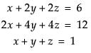
A = [1 2 2, 2 4 4, 1 1 1];
B = [6, 12, 1];
Show( GInverse( A ) * B );
GInverse(A) * B = [-4, 2.5, 2.5];
The Solve() function solves a system of linear equations. Solve() finds the vector x so that x = A-1b where A equals a square, nonsingular matrix and b is a vector. The matrix A and the vector b must have the same number of rows. Solve(A,b) is the same as Inverse(A)*b.
A = [1 -4 2, 3 3 2, 0 4 -1];
b = [1, 2, 1];
x = Solve( A, b );
[-16.9999999999999, 4.99999999999998, 18.9999999999999]
A*x;
[1, 2, 0.999999999999997]
The Sweep() function inverts parts (or pivots) of a square matrix. If you sequence through all of the pivots, you are left with the matrix inverse. Normally the matrix must be positive definite (or negative definite) so that the diagonal pivots never go to zero. Sweep() does not check whether the matrix is positive definite. If the matrix is not positive definite, then it still works, as long as no zero pivot diagonals are encountered. If zero (or near-zero) diagonal pivots are encountered on a full sweep, then the result is a g2 generalized inverse if the zero pivot row and column are zeroed.

The syntax for Sweep() appears as follows:
Sweep( E, [...] );
|
•
|
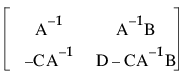
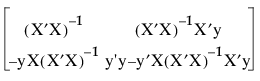
The submatrix in the A position becomes the inverse.
|
|
•
|
|
•
|
Sweep() is sequential and reversible:
|
•
|
A = Sweep( A, {i,j} ) is the same as A = Sweep( Sweep( A, i ), j ). It is sequential.
|
|
•
|
A = Sweep( Sweep( A, i ), i ) restores A to its original values. It is reversible.
|
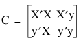
Then after sweeping through the indices of X’X, the result appears as follows:
|
•
|
the least squares estimates for the model Y = Xb + e in the upper right
|
The Sweep function is useful in computing the partial solutions needed for stepwise regression.
The index argument is a vector that lists the rows (or equivalently the columns) on which you want to sweep the matrix. For example, if E is a 4x4 matrix, to sweep on all four rows to get E-1 requires these commands:
E = [ 5 4 1 1, 4 5 1 1, 1 1 4 2, 1 1 2 4];
Sweep( E, [1, 2, 3, 4] );
[0.56 -0.44 -0.02 -0.02,
-0.44 0.56 -0.02 -0.02,
-0.02 -0.02 0.34 -0.16,
-0.02 -0.02 -0.16 0.34]
Inverse( E ); // notice that these results are the same
[0.56 -0.44 -0.02 -0.02,
-0.44 0.56 -0.02 -0.02,
-0.02 -0.02 0.34 -0.16,
-0.02 -0.02 -0.16 0.34]
Note: For a tutorial on Sweep(), and its relation to the Gauss-Jordan method of matrix inversion, see Goodnight, J.H. (1979) “A tutorial on the SWEEP operator.” The American Statistician, August 1979, Vol. 33, No. 3. pp. 149–58.
Sweep() is further demonstrated in the ANOVA Example.
The Det() function returns the determinant of a square matrix. The determinant of a 2 × 2 matrix is the difference of the diagonal products, as demonstrated below. Determinants for n × n matrices are defined recursively as a weighted sum of determinants for (n - 1) × (n - 1) matrices. For a matrix to have an inverse, the determinant must be nonzero.
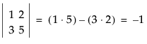
F = [1 2, 3 5];
Det( F );
-1