Y = [98, 112.5, 84, 102.5, 102.5, 50.5, 90, 77, 112, 150, 128, 133, 85, 112];
X = [65.3, 69, 56.5, 62.8, 63.5, 51.3, 64.3, 56.3, 66.5, 72, 64.8, 67, 57.5, 66.5];
X = J( N Row( X ), 1 ) || X; // put in an intercept column of 1s
beta = Inv( X` * X ) * X` * Y; // the least square estimates
resid = Y - X * beta; // the residuals, Y - predicted
sse = resid` * resid; // sum of squared errors
Show( beta, sse );
// open the data table
dt = Open( "$SAMPLE_DATA/Big Class.jmp" );
// get data into matrices
x = (Column( "Age" ) << Get Values ) || (Column( "Height" ) << Get Values);
x = J(N Row( x ), 1, 1) || x;
y = Column( "Weight" ) << Get Values;
// regression calculations
xpxi = Inv( x` * x );
beta = xpxi * x` * y; // parameter estimates
resid = y - x * beta; // residuals
sse = resid` * resid; // sum of squared errors
dfe = N Row( x ) - N Col( x ); // degrees of freedom
mse = sse / dfe; // mean square error, error variance estimate
// additional calculations on estimates
stdb = Sqrt( Vec Diag( xpxi ) * mse ); // standard errors of estimates
alpha = .05;
qt = Students t Quantile( 1 - alpha / 2, dfe );
betau95 = beta + qt * stdb; // upper 95% confidence limits
betal95 = beta - qt * stdb; // lower 95% confidence limits
tratio = beta :/ stdb; // Student's T ratios
probt = ( 1 - TDistribution( Abs( tratio ), dfe ) ) * 2; // p-values
// present results
New Window( "Big Class Regression",
Table Box(
String Col Box( "Term",{"Intercept", "Age", "Height"} ),
Number Col Box( "Estimate", beta ),
Number Col Box( "Std Error", stdb ),
Number Col Box( "TRatio", tratio ),
Number Col Box( "Prob>|t|", probt ),
Number Col Box( "Lower95%", betal95 ),
Number Col Box( "Upper95%", betau95 ) ) );
|
•
|
Y is a vector of responses
|
|
•
|
a is the intercept term
|
|
•
|
b is a vector of coefficients
|
|
•
|
X is a design matrix for the factor
|
|
•
|
e is an error term
|
factor = [1, 2, 3, 1, 2, 3, 1, 2, 3];
y = [1, 2, 3, 4, 3, 2, 5, 4, 3];
Design Nom( factor );
[1 0, 0 1, -1 -1, 1 0, 0 1, -1 -1, 1 0, 0 1, -1 -1]
Next, add a column of 1s to the design matrix for the intercept term. You can do this by concatenating J and Design Nom(), as follows:
x = J( 9, 1, 1) || Design Nom( factor );
[1 1 0,
1 0 1,
1 -1 -1,
1 1 0,
1 0 1,
1 -1 -1,
1 1 0,
1 0 1,
1 -1 -1]
Now, to solve the normal equation, you need to construct a matrix M with partitions:

You can construct matrix M in one step by concatenating the pieces, as follows:
M = ( x` * x || x` * y )
|/
( y` * x || y` * y );
[9 0 0 27,
0 6 3 2,
0 3 6 1,
27 2 1 93]
Now, sweep M over all the columns in X’X for the full fit model, and over the first column only for the intercept-only model:
FullFit = Sweep( M, [1, 2, 3] ); // full fit model
InterceptOnly = Sweep( M, [1] ); // model with intercept only
[0.111111111111111 0 0 3,
0 0.222222222222222 -0.11111111111111 0.333333333333333,
0 -0.11111111111111 0.222222222222222 0,
-3 -0.33333333333333 0 11.33333333333333]
|
•
|
You could modify this into a generalized ANOVA script by replacing some of the explicit values in the script with arguments. These results match those from the Fit Model platform. See Figure 6.1.
Figure 6.1 ANOVA Report Within Fit Model
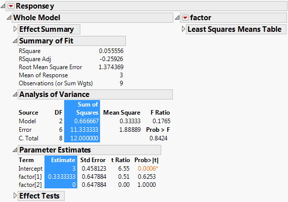
Construct the report in Figure 6.1 as follows:
dt = New Table( "Data" );
dt << New Column( "y", Set Values( [1, 2, 3, 4, 3, 2, 5, 4, 3] ) );
dt << New Column( "factor", "Nominal", Values( [1, 2, 3, 1, 2, 3, 1, 2, 3] ) );
|
2.
|
obj = Fit Model(
Y( :y ),
Effects( :factor ),
Personality( "Standard Least Squares" ),
Run(
y << {Plot Actual by Predicted( 0 ), Plot Residual by Predicted( 0 ),
Plot Effect Leverage( 0 )}
)
);
|
3.
|
ranova = obj << Report;
ranova[Outline Box( 6 )] << Close( 0 );
ranova[Outline Box( 7 )] << Close( 1 );
ranova[Outline Box( 9 )] << Close( 1 );
ranova[Outline Box( 5 ), Number Col Box( 2 )] << Select;
ranova[Outline Box( 6 ), Number Col Box( 1 )] << Select;