|
1.
|
Select File > New > Data Table.
|
|
2.
|
|
3.
|
Change the column name to Run Order.
|
|
4.
|
|
5.
|
Type 16 next to To.
|
|
6.
|
Click OK.
|
|
7.
|
Select DOE > Custom Design.
|
|
8.
|
Click Add Factor > Covariate.
|
|
9.
|
|
10.
|
Type 7 next to Add N Factors.
|
|
11.
|
Click Add Factor > Continuous.
|
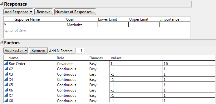
Figure 4.68 Responses and Factors Outlines
|
12.
|
Click Continue.
|
|
13.
|
Open the Alias Terms outline.
|
|
14.
|
Select all of the effects in the list and click Remove Term.
|
Note: Setting the Random Seed in step 15 and Number of Starts in step 16 reproduces the exact results shown in this example. In constructing a design on your own, these steps are not necessary.
|
15.
|
(Optional) From the Custom Design red triangle menu, select Set Random Seed, type 1084680980, and click OK.
|
|
16.
|
(Optional) From the Custom Design red triangle menu, select Number of Starts, type 30000, and click OK.
|
|
17.
|
Click Make Design.
|
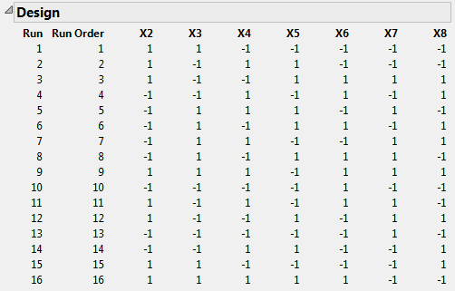
Figure 4.69 Design Outline
|
18.
|
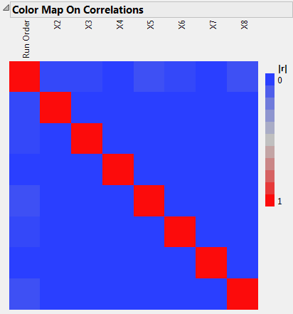
Open the Design Evaluation > Color Map On Correlations outline.
|
|
–
|
|
–
|
Run Order, the linear time trend variable, has extremely low absolute correlation with X2 through X8.
|
|
19.
|
Open the Design Evaluation > Estimation Efficiency outline.
|
Figure 4.71 Estimation Efficiency Outline
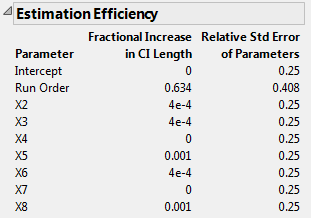
The small absolute correlations of Run Order with X2 through X8 result in very small increases in confidence interval lengths, relative to an ideal orthogonal design. The increases in the lengths of confidence intervals for X2 through X8 are all less than 0.1%.