Use this option to obtain tests and confidence levels that compare means defined by levels of your model effects. The goal of multiple comparisons methods is to determine whether group means differ, while controlling the probability of reaching an incorrect conclusion. The Multiple Comparisons option lets you compare group means with the overall average (Analysis of Means) and with a control group mean. You can also conduct pairwise comparisons using either Tukey HSD or Student’s t. When you specify the Student’s t method, you can also perform equivalence tests to identify pairwise differences that are of practical importance.
The Student’s t method controls only the error rate for an individual comparison. As such, it is not a true multiple comparison procedure. All other methods provided control the overall error rate for all comparisons of interest. Each of these methods uses a multiple comparison adjustment in calculating p-values and confidence limits.
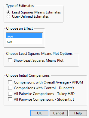
An example of the control window for the Multiple Comparisons option is shown in Figure 2.28. This example is based on the Big Class.jmp data table, with weight as Y and age, sex, and height as model effects. Two classes of estimates are available for comparisons: Least Squares Means Estimates and User-Defined Estimates.
This option compares least squares means and is available only if there are nominal or ordinal effects in the model. Recall that least squares means are means computed at some neutral value of the other effects in the model. (For a definition of least squares means, see LSMeans Table.) You must select the effect of interest. In Figure 2.28, Least Squares Means Estimates for age are specified. There is an option to show the least squares means plot. See Least Squares Means Plot Options.
Figure 2.28 Launch Window for Least Squares Means Estimates
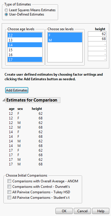
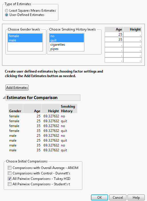
The specification of User-Defined Estimates is illustrated in Figure 2.29. Three levels of age and both levels of sex have been selected. Also, two values of height have been manually entered. The Add Estimates button has been clicked, resulting in the listing of all possible combinations of the specified levels. At this point, you can specify more estimates and click the Estimates button again to add them to the list of Estimates for Comparison.
Figure 2.29 Launch Window for User-Defined Estimates
Note: In this section, we use the term mean to refer to either estimates of least squares means or user-defined estimates.
Select Show Least Squares Means Plot to obtain a least square means plot. If your effect is an interaction term, then you have the option to create an interaction plot. You select the term for the overlay. If you do not select the interaction plot, then the least squares plot will nest the effect terms. See Least Squares Means Plot Options.
The t ratio for the significance test. This column appears only if you right-click in the report and select Columns > t Ratio.
The p-value for the significance test. This column appears only if you right-click in the report and select Columns > Prob>|t|.
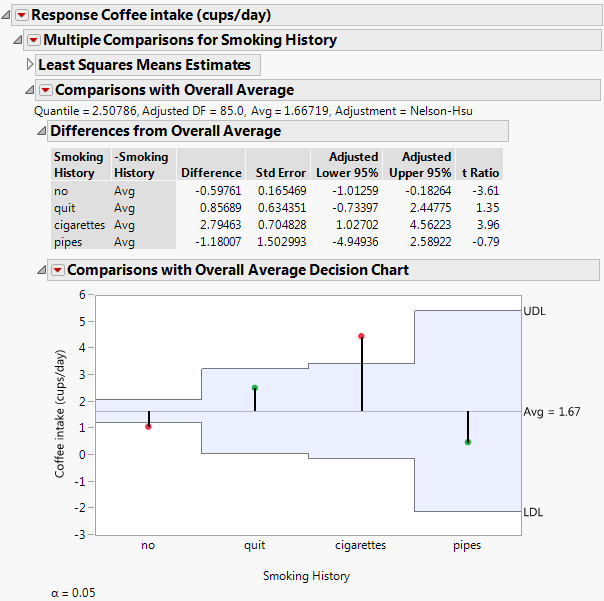
This option compares the means for the specified levels specified to the overall mean for these levels. It displays a table showing confidence intervals for differences from the overall mean and a chart showing decision limits. The method used to make the comparisons is called analysis of means (ANOM) (Nelson et al. 2005). ANOM is a multiple comparison procedure that controls the joint error rate for all pairwise comparisons to the overall mean. See Figure 2.30 for a report based on the Lipid Data.jmp sample data table.
The value of Nelson’s h statistic used in constructing the decision limits.
Specifically, the average least squares mean is a weighted average with weights inversely proportional to the diagonal entries of the matrix  . Here L is the matrix of coefficients used to compute the group least squares means. For a technical definition of least squares means and the average least squares mean, see the GLM Procedure chapter in the SAS/STAT 14.3 User’s Guide (SAS Institute Inc. 2017).
. Here L is the matrix of coefficients used to compute the group least squares means. For a technical definition of least squares means and the average least squares mean, see the GLM Procedure chapter in the SAS/STAT 14.3 User’s Guide (SAS Institute Inc. 2017).For user-defined estimates, the average mean is defined similarly. However, in this case, L is the matrix of coefficients used to define the estimates.
|
–
|
Nelson: Provides exact critical values and p-values. Used whenever possible, in particular, when the estimates are uncorrelated.
|
|
–
|
Nelson-Hsu: Provides approximate critical values and p-values based on Hsu’s factor analytical approximation is used (Hsu 1992). Used when exact values cannot be obtained.
|
For technical details, see the GLM Procedure chapter in the SAS/STAT 14.3 User’s Guide (SAS Institute Inc. 2017).
Adds a column that contains p-values (Prob>|t|) to the Comparisons with Overall Average report. Note that computing exact critical values and p-values for unbalanced designs requires complex integration and can be computationally challenging. When calculations for such a quantile fail, the Sidak quantile is computed but p-values are not available.
Consider the Lipid Data.jmp sample data table. You are interested in whether any of the four Smoking History categories are unusual in that their mean Coffee intake (cups/day) differ from the overall average coffee intake while controlling for alcohol use and heart history. You specify a model with Coffee intake (cups/day) as the response and Smoking History, Alcohol Use, and Heart History as model effects.
|
1.
|
|
2.
|
Select Analyze > Fit Model.
|
|
3.
|
|
4.
|
|
5.
|
Click Run.
|
|
6.
|
From the red triangle next to Response Coffee intake (cups/day), select Estimates > Multiple Comparisons.
|
|
7.
|
From the Choose an Effect list, select Smoking History.
|
|
8.
|
In the Choose Initial Comparisons list, select Comparisons with Overall Average - ANOM.
|
|
9.
|
Click OK.
|
The results shown in Figure 2.30 indicate that the least squares means for non-smokers and cigarette smokers differ significantly from the overall average in terms of coffee intake.
Figure 2.30 Comparisons with Overall Average for Ratings
After you choose a control group and click OK, the Comparisons with Control report appears in your Fit Least Squares report. This option compares the means for the specified settings to the control group mean. It displays a table showing confidence intervals for differences from the control group and a chart showing decision limits. Dunnett’s method is used to make the comparisons. Dunnett’s method is a multiple comparison procedure that controls the error rate over all comparisons (Hsu 1996; Westfall et al. 2011).
When exact calculation of p-values and confidence intervals is not possible, Hsu’s factor analytical approximation is used (Hsu 1992). Note that computing exact critical values and p-values for unbalanced designs requires complex integration and can be computationally intensive. When calculations for such a quantile fail, the Sidak quantile is computed.
|
–
|
Dunnett: Provides exact critical values and p-values. Used whenever possible, in particular, when the estimates are uncorrelated.
|
|
–
|
Dunnett-Hsu: Provides approximate critical values and p-values based on Hsu’s factor analytical approximation (Hsu 1992). Used when exact values cannot be obtained.
|
For technical details, see the GLM Procedure chapter in the SAS/STAT 14.3 User’s Guide (SAS Institute Inc. 2017).
For each comparison of a group mean to the control mean, this report provides the following details:
Adds a column that contains p-values (Prob>|t|) to the Comparisons with Control report. Note that computing exact critical values and p-values for unbalanced designs requires complex integration and can be computationally challenging. When calculations for such a quantile fail, the Sidak quantile is computed but p-values are not available.
The All Pairwise Comparisons option shows either a Tukey HSD All Pairwise Comparisons or Student’s t All Pairwise Comparisons report (Hsu 1996; Westfall et al. 2011). Tukey HSD comparisons are constructed so that the significance level applies jointly to all pairwise comparisons. In contrast, for Student’s t comparisons, the significance level applies to each individual comparison. When making several pairwise comparisons using Student’s t tests, the risk that one of the comparisons incorrectly signals a difference can well exceed the stated significance level.
The critical value for the test. Note that, for Tukey HSD, the quantile is  , where q is the appropriate percentage point of the Studentized range statistic.
, where q is the appropriate percentage point of the Studentized range statistic.|
–
|
Tukey: Provides exact critical values and p-values. Used when the means are uncorrelated and have equal variances, or when the design is variance-balanced.
|
|
–
|
Tukey-Kramer: Provides approximate critical values and p-values. Used when exact values cannot be obtained.
|
For technical details, see the GLM Procedure chapter in the SAS/STAT 14.3 User’s Guide (SAS Institute Inc. 2017).
At the top of the Student’s t All Pairwise Comparisons report you find the Quantile, or critical value, for the t test and DF, the degrees of freedom used for the t test.
Both Tukey HSD and Student’s t compare all pairs of levels. For each pairwise comparison, the All Pairwise Differences report shows:
|
•
|
t Ratio - the t ratio for the test of whether the difference is zero
|
|
•
|
Prob > |t| - the p-value for the test
|
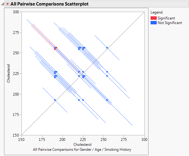
This plot, sometimes called a diffogram or a mean-mean scatterplot, displays the confidence intervals for all means pairwise differences. (See Figure 2.32 for an example.) Colors indicate which differences are significant.
Use this option to conduct one or more equivalence tests. Equivalence tests are useful when you want to detect differences that are of practical interest. You are asked to specify a threshold difference for group means for which smaller differences are considered practically equivalent. In other words, if two group means differ by this amount or less, you are willing to consider them equivalent.
The Two One-Sided Tests (TOST) method is used to test for a practical difference between the means (Schuirmann 1987). Two one-sided pooled-variance t tests are constructed for the null hypotheses that the true difference exceeds the threshold values. If both tests reject, the difference in the means does not statistically exceed either threshold value. Therefore, the groups are considered practically equivalent. If only one or neither test rejects, then the groups might not be practically equivalent.
|
•
|
Lower Bound t Ratio, Upper Bound t Ratio - the lower and upper bound t ratios for the two one-sided pooled-variance significance tests
|
|
•
|
Lower Bound p-Value, Upper Bound p-value - p-values corresponding to the lower and upper bound t ratios
|
 confidence interval for the difference in the means.
 confidence interval for a pairwise comparison. The coordinates of the point on the line segment are the means for the corresponding groups. Placing your cursor over one of these points displays a tooltip indicating the groups being compared and the estimated difference. When a line segment is entirely contained within the diagonal band, it follows that the means are practically equivalent.
Consider the Lipid Data.jmp sample data table. You are interested in Cholesterol differences for gender and non-smokers versus former smokers (Smoking History equal to no and quit, respectively) across two ages (25 and 35) and average height.
|
1.
|
|
2.
|
Select Analyze > Fit Model.
|
|
3.
|
|
4.
|
|
5.
|
Click Run.
|
|
6.
|
From the red triangle next to Response Cholesterol, select Estimates > Multiple Comparisons.
|
|
7.
|
From the Type of Estimates list, click User-Defined Estimates.
|
|
8.
|
From the Choose Gender levels list, select female (it should already be selected by default) and male.
|
|
9.
|
|
10.
|
In the Age list, enter the ages 25 and 35 in the first two rows.
|
Do not enter any values in the list entitled Height. Because no values for Height are specified, the mean value of the Height column is used in the multiple comparisons report.
|
11.
|
Click Add Estimates.
|
|
12.
|
In the Choose Initial Comparisons list, select All Pairwise Comparisons - Tukey HSD.
|
Figure 2.31 Populated Used-Defined Estimates Window
|
13.
|
Click OK.
|
The All Pairwise Differences report indicates that two of the 28 pairwise comparisons are significant. The All Pairwise Comparisons Scatterplot, shown in Figure 2.32, shows the confidence intervals for these comparisons in red. You can place your pointer over any of the points to determine which pairwise comparison the point represents. The tooltips also contain the difference between the two levels in the comparison. The two red points in Figure 2.32 represent the points comparing 35-year-old former smokers to 25-year-old non-smokers, for both females and males.