Response Surface Design

The following example contains these sections:

•

Construct a response surface design for three continuous factors that you have identified as active. You want to find process settings to maintain your response(Y) within specifications. The lower and upper specification limits for Y are 54 and 56, respectively, with a target of 55.

Select DOE > Custom Design.

In the Responses outline, click Maximize and select Match Target.

Type 54 as the Lower Limit and 56 as the Upper Limit.

Leave Importance blank.

Because there is only one response, the Importance value is set to 1 by default.

Type 3 next to Add N Factors.

Click Add Factor > Continuous.

This adds three continuous factors: X1, X2, and X3.

Click Continue.

In the Model outline, click the RSM button.

This adds quadratic and interaction terms to the model. It also sets the value of the Recommended optimality criterion to I-optimality. You can verify this in the Design Diagnostics outline once you click Make Design.

Leave the Default Number of Runs set to 16.

Note: Setting the Random Seed in step 9 and Number of Starts in step 10 reproduces the exact results shown in this example. In constructing a design on your own, these steps are not necessary.

(Optional) From the Custom Design red triangle menu, select Set Random Seed, type 929281409, and click OK.

10.

(Optional) From the Custom Design red triangle menu, select Number of Starts, type 40, and click OK.

11.

Click Make Design.

The Design outline shows the design.

Figure 4.26 RSM Design

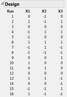
In order to estimate quadratic effects, a response surface design uses three levels for each factor. Note that the design in Figure 4.26 is a face-centered Central Composite Design with two center points.

12.

Open the Design Evaluation > Design Diagnostics outline.

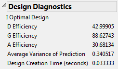
Figure 4.27 Design Diagnostics Outline

The first line in the Design Diagnostics outline identifies the optimality criterion being used. This design is I-optimal.

13.

Open the Design Evaluation > Prediction Variance Profile outline.

Figure 4.28 Prediction Variance Profile

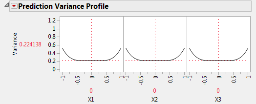
The vertical axis shows the relative prediction variance of the expected value of the response. The relative prediction variance is the prediction variance divided by the error variance. When the relative prediction variance is one, its absolute variance equals the error variance of the regression model.

The profiler shows values of the relative prediction variance over the design space. You can move the sliders to explore the prediction variance’s behavior. The prediction variance is smallest in the center of the design space. It is fairly constant, with values only slightly larger than 0.2, for factor settings between -0.5 and 0.5. The prediction variance increases as the settings approach the design space boundaries.

14.

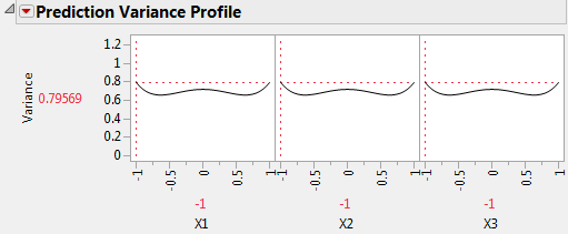
Select Maximize Variance from the red triangle menu next to Prediction Variance Profile outline.

Figure 4.29 Prediction Variance Profile with Relative Variance Maximized

The profiler shows that the maximum value of the relative prediction variance is 0.79569.

15.

Open the Design Evaluation > Fraction of Design Space Plot outline.

Figure 4.30 Fraction of Design Space Plot

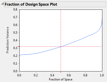
The blue curve in the plot shows the relative prediction variance as a function of the fraction of design space. The red dashed cross hairs indicate that, for 50% of the design space, the prediction variance is about 0.32 or less. Use the cross hair tool to draw other inferences. For example, when the Fraction of Space is 0.95, the Prediction Variance is about 0.52. This means that for 95% of the design space, the relative prediction variance is below 0.52.

Analyze the Experimental Results

The Custom RSM.jmp sample data table contains the results of the experiment. The Model script opens a Fit Model window showing all of the effects specified in the DOE window’s Model outline. This script was saved to the data table by the Custom Design platform.

Select Help > Sample Data Library and open Design Experiment/Custom RSM.jmp.

In the Table panel, click the green triangle next to the Model script.

Click Run.

The Effect Summary report shows the LogWorth and PValue for each effect in the model. The vertical blue line in the plot is set at the value 2. A LogWorth that exceeds 2 is significant at the 0.01 level.

Figure 4.31 Effect Summary Report

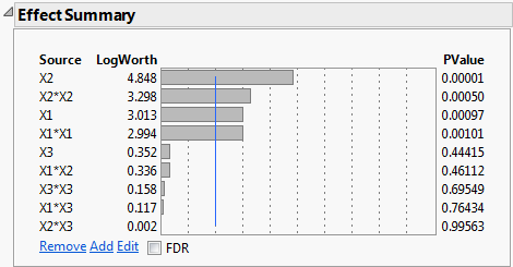
The report shows that X1, X2, X1*X1, and X2*X2 are significant at the 0.01 level. None of the other effects are significant at even the 0.10 level. Reduce the model by removing these insignificant effects.

In the Effect Summary report, select X3, X1*X2, X3*X3, X1*X3, and X2*X3.

Figure 4.32 Effect Summary Report with Insignificant Effects Selected

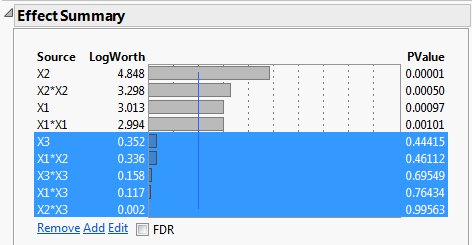
Click Remove.

The Fit Least Squares report is updated to show a model containing only the significant effects: X1, X2, X1*X1, and X2*X2.

Use the Prediction Profiler (at the bottom of the Fit Least Squares window) to explore how the predicted response (Y) changes as you vary the factors X1 and X2. Note the quadratic behavior of Y across the values of X1 and X2.

Remember that you entered response limits for Y in the Responses outline of the Custom Design window. As a result, the Response Limit column property is attached to the Y column in the design table. The Desirability function for Y (in the top plot at right) is based on the information contained in the Response Limit column property. JMP uses this function to calculate Desirability as a function of the settings of X1 and X2. The traces of the Desirability function appear in the bottom row of plots.

In the Prediction Profiler report, select Optimization and Desirability > Maximize Desirability from the red triangle options.

Figure 4.33 Prediction Profiler with Desirability Maximized

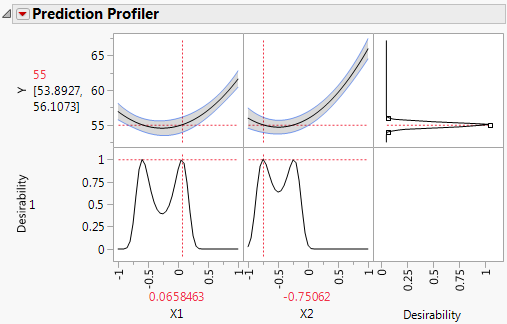
The predicted response achieves the target value of 55 at the process settings shown in red above X1 and X2. Figure 4.33 shows that a value of X1 near –0.65 also achieves a predicted value of 55 when X2 = -0.75062. In fact, your Prediction Profiler might show different settings as those that maximize desirability. This is because the predicted response is 55 for many settings of X1 and X2.

Select Factor Profiling > Contour Profiler from the red triangle next to Response Y.

In the Contour Profiler report, type 55 as the value for Contour.

Figure 4.34 Contour Profiler

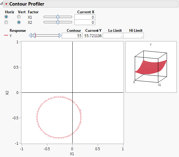
The settings of X1 and X2 that correspond to the red contour have predicted response values of 55. You might want to select from among these process settings based on cost efficiency.