Continuing with the Drug.jmp sample data table, this example fits a model where the slope for the covariate depends on the level of Drug.
|
1.
|
|
2.
|
Select Analyze > Fit Model.
|
|
3.
|
|
4.
|
This adds terms up to the degree specified in the Degree box to the model. The default value for Degree is 2. Thus the main effects of Drug and x, and their interaction, Drug*x, are added to the model effects list.
|
5.
|
Click Run.
|
This specification adds two columns to the linear model (call them x4i and x5i) that allow the slopes for the covariate to differ by Drug level. The new variables are formed by multiplying the indicator variables for Drug by the covariate values, giving the following formula:
Coding of Analysis of Covariance with Separate Slopes, shows the coding for this model. The mean of X, which is 10.7333, is used in centering continuous terms.
|
X1
|
||
|
X2
|
||
|
X3
|
||
|
X4
|
X – 10.7333 if a, 0 if d, –(X – 10.7333) if f
|
|
|
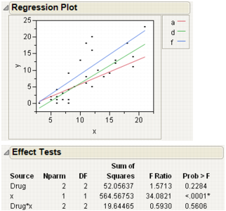
X5
|
A portion of the report is shown in Plot with Interaction. The Regression Plot shows fitted lines with different slopes. The Effect Tests report gives a p-value for the interaction of 0.56. This is not significant, indicating the model does not need to include different slopes.