This example constructs a response surface model using the Odor Control Original.jmp file in the Sample Data folder. The objective is to find the range of temperature (temp), gas-liquid ratio (gl ratio), and height (ht) values that minimize the odor of a chemical production process.
|
1.
|
|
2.
|
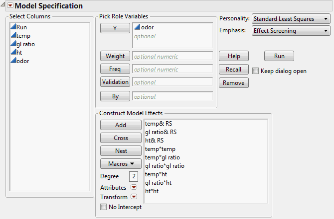
Select Analyze > Fit Model.
|
|
3.
|
|
4.
|
This Macro adds terms up to degree two to the model (Fit Model Dialog for Response Surface Analysis). The main effects appear in the Construct Model Effects list with a &RS suffix. As a result, the analysis results will include a Response Surface report.
|
5.
|
Click Run.
|
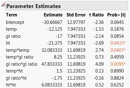
The Parameter Estimates table shows estimates of the model parameters (Parameter Estimates Table). Two of the quadratic effects, gl ratio*gl ratio and temp*temp, as well as the main effect of ht, are significant at the 0.05 level.
|
6.
|
From the report’s red triangle menu, select Save Columns > Prediction Formula.
|
This inserts a column into the data table called Pred Formula odor. This column contains the prediction formula defined by the coefficients shown in the Parameter Estimates table.
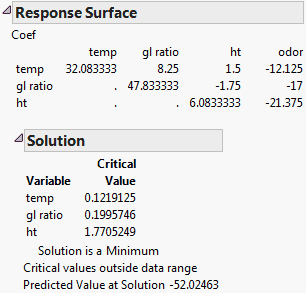
A response surface report is provided (Response Surface Report). This report shows a table showing the second-order model coefficients in matrix form. The Solution report shows the critical values for the main effects. These are the values where a maximum, a minimum, or a saddle point occur. The Solution report indicates which of these occurs at the critical point. In this example, the response surface achieves a minimum at the critical value.
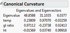
The Response Surface report also contains the Canonical Curvature subreport (Basic Reports for Response Surface Model). This report shows the eigenstructure of the matrix of second-order parameter estimates. The eigenstructure is useful for identifying the shape and orientation of the curvature. The eigenvalues, given in the first row of the Canonical Curvature table, are negative if the response surface curves down from a maximum. The eigenvalues are positive if the surface curves up from a minimum. If the eigenvalues are mixed, the surface is saddle shaped, curving up in one direction and down in another direction.
The eigenvectors listed beneath the eigenvalues show the orientations of the principal axes. In this example the eigenvalues are positive, which indicates that the surface achieves a minimum. The direction of greatest curvature corresponds to the largest eigenvalue (48.8588). That direction is defined by the corresponding eigenvector components. For the first direction, gl ratio, with an eigenvector value of 0.97112, has the greatest influence. The direction defined by the eigenvalue of 31.1035 is determined more by temp (0.97070), than by gl ratio or ht.
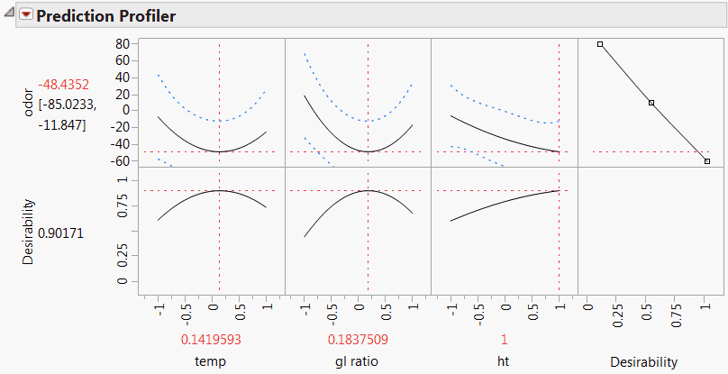
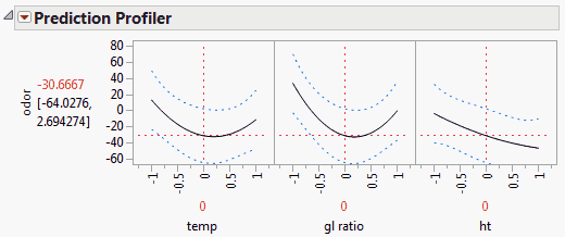
The Prediction Profiler report, at the bottom of the results window, shows the quadratic behavior of the response surface along traces for temp and gl ratio (Prediction Profiler).
|
7.
|
From the Prediction Profiler’s red triangle menu, select Desirability Functions.
|
In the top row for odor, to the far right, a cell that plots the desirability function is added. A row of cells showing desirability traces is added beneath the row for odor.
|
9.
|
In the drop-down list, select Minimize.
|
|
10.
|
Click OK.
|
|
11.
|
From the Prediction Profiler’s red triangle menu, select Maximize Desirability.
|
Settings within the design region that minimize odor are shown beneath the profiler (Prediction Profiler with Desirability Function Optimized).