Using the Fit Line command, you can add straight line fits to your scatterplot using least squares regression. Using the Fit Polynomial command, you can fit polynomial curves of a certain degree using least squares regression.
Example of Fit Line and Fit Polynomial shows an example that compares a linear fit to the mean line and to a degree 2 polynomial fit.
|
•
|
The Fit Line output is equivalent to a polynomial fit of degree 1.
|
|
•
|
The Fit Mean output is equivalent to a polynomial fit of degree 0.
|
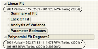
Each Linear and Polynomial Fit Degree report contains at least three reports. A fourth report, Lack of Fit, appears only if there are X replicates in your data.
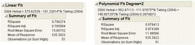
The Summary of Fit reports show the numeric summaries of the response for the linear fit and polynomial fit of degree 2 for the same data. You can compare multiple Summary of Fit reports to see the improvement of one model over another, indicated by a larger Rsquare value and smaller Root Mean Square Error.
|
Measures the proportion of the variation explained by the model. The remaining variation is not explained by the model and attributed to random error. The Rsquare is 1 if the model fits perfectly.
The Rsquare values in Summary of Fit Reports for Linear and Polynomial Fits indicate that the polynomial fit of degree 2 gives a small improvement over the linear fit.
|
|
|
Adjusts the Rsquare value to make it more comparable over models with different numbers of parameters by using the degrees of freedom in its computation.
|
|
|
Estimates the standard deviation of the random error. It is the square root of the mean square for Error in the Analysis of Variance report. See Examples of Analysis of Variance Reports for Linear and Polynomial Fits.
|
|
Using the Lack of Fit report, you can estimate the error, regardless of whether you have the right form of the model. This occurs when multiple observations occur at the same x value. The error that you measure for these exact replicates is called pure error. This is the portion of the sample error that cannot be explained or predicted no matter what form of model is used. However, a lack of fit test might not be of much use if it has only a few degrees of freedom for it (few replicated x values).
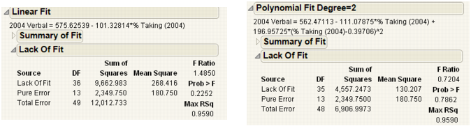
The difference between the residual error from the model and the pure error is called the lack of fit error. The lack of fit error can be significantly greater than the pure error if you have the wrong functional form of the regressor. In that case, you should try a different type of model fit. The Lack of Fit report tests whether the lack of fit error is zero.
|
The degrees of freedom (DF) for each source of error.
|
|||||||
|
|||||||
|
The sum of squares divided by its associated degrees of freedom. This computation converts the sum of squares to an average (mean square). F-ratios for statistical tests are the ratios of mean squares.
|
|||||||
|
The probability of obtaining a greater F-value by chance alone if the variation due to lack of fit variance and the pure error variance are the same. A high p value means that there is not a significant lack of fit.
|
|||||||
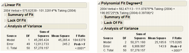
Analysis of variance (ANOVA) for a regression partitions the total variation of a sample into components. These components are used to compute an F-ratio that evaluates the effectiveness of the model. If the probability associated with the F-ratio is small, then the model is considered a better statistical fit for the data than the response mean alone.
The Analysis of Variance reports in Examples of Analysis of Variance Reports for Linear and Polynomial Fits compare a linear fit (Fit Line) and a second degree (Fit Polynomial). Both fits are statistically better from a horizontal line at the mean.
|
|||||||
|
|||||||
|
The sum of squares divided by its associated degrees of freedom. The F-ratio for a statistical test is the ratio of the following mean squares:
|
|||||||
|
The model mean square divided by the error mean square. The underlying hypothesis of the fit is that all the regression parameters (except the intercept) are zero. If this hypothesis is true, then both the mean square for error and the mean square for model estimate the error variance, and their ratio has an F-distribution. If a parameter is a significant model effect, the F-ratio is usually higher than expected by chance alone.
|
|||||||
|
The observed significance probability (p-value) of obtaining a greater F-value by chance alone if the specified model fits no better than the overall response mean. Observed significance probabilities of 0.05 or less are often considered evidence of a regression effect.
|
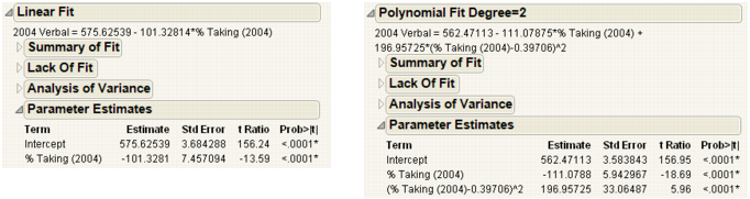
The terms in the Parameter Estimates report for a linear fit are the intercept and the single x variable.
For a polynomial fit of order k, there is an estimate for the model intercept and a parameter estimate for each of the k powers of the X variable.
|
Lists the observed significance probability calculated from each t-ratio. It is the probability of getting, by chance alone, a t-ratio greater (in absolute value) than the computed value, given a true null hypothesis. Often, a value below 0.05 (or sometimes 0.01) is interpreted as evidence that the parameter is significantly different from zero.
|
To reveal additional statistics, right-click in the report and select the Columns menu. Statistics not shown by default are as follows:
The standardized parameter estimate. It is useful for comparing the effect of X variables that are measured on different scales. See Statistical Details for the Parameter Estimates Report.