|
•
|
A matrix with one row or one column is a vector (or more specifically, a row vector or a column vector respectively).
|
|
•
|
A scalar is a numeric value that is not in a matrix.
|
Create matrix A with 3 rows and 2 columns:
R is a row vector and C is a column vector:
B is a 1-by-1 matrix, or a matrix with one row and one column:
E is an empty matrix:
A script can return an empty matrix. In Big Class.jmp, the following expression looks for rows in which age equals 8, finds none, and returns an empty matrix:
If you want to convert lists into a matrix, use the Matrix() function. A single list is converted into a column vector. Two or more lists are converted into rows.
To construct matrices from expressions, use Matrix(). Elements must be expressions that resolve to numbers.
Use the subscript operator ([ ]) to pick out elements or submatrices from matrices. The Subscript() function is usually written as a bracket notation after the matrix to be subscripted, with arguments for rows and columns.
The expression A[i,j] extracts the element in row i, column j, returning a scalar number. The equivalent functional form is Subscript(A,i,j).
Assign the value that is in the third row and the first column in the matrix A (which is 5) to the variable test.
A single subscript addresses matrices as if all the rows were connected end-to-end in a single row. This makes the double subscript A[i,j] the same as the single subscript A[(i-1)*ncol(A)+j].
You can use operator assignments (such as +=) on matrices or subscripts of matrices. For example, the following statement adds 1 to the i - jth element of the matrix:
If you are working with a range of subscripts, use the Index() function :: to create matrices of ranges.
The NCol() and NRow() functions return the number of columns and rows in a matrix (or data table), respectively:
To determine whether a value is a matrix, use the Is Matrix() function, which returns a 1 if the argument evaluates to a matrix.
You can use the Any() or All() operators to summarize matrix comparison results. Any() returns a 1 if any element is nonzero. All() returns a 1 if all elements are nonzero.
Min() or Max() return the minimum or maximum element from the matrix or matrices given as arguments.
|
•
|
|
•
|
* operator
|
|
•
|
Multiply() function
|
|
•
|
Matrix Mult() function
|
|
•
|
/ operator
|
|
•
|
Divide() function
|
|
•
|
|
•
|
|
•
|
Matrix division (equivalent to A*Inverse(D)):
|
•
|
|
•
|
|
•
|
|
•
|
Normal Distribution(), and other probability functions.
|
The Concat() function combines two matrices side by side to form a larger matrix. The number of rows must agree. A double vertical bar ( || ) is the infix operator, equivalent for horizontal concatenation.
The VConcat() function stacks two matrices on top of each other to form a larger matrix. The number of columns must agree. A vertical-bar-slash ( |/ ) is the infix operator, equivalent for vertical concatenation.
There are two in place concatenation operators: ||= and |/= . They are equivalent to the Concat To()and V Concat To() functions, respectively.
|
•
|
a||=b is equivalent to a=a||b
|
|
•
|
a|/=b is equivalent to a=a|/b
|
The Transpose() function transposes the rows and columns of a matrix. A back-quote ( ` ) is the postfix operator, equivalent to Transpose(). In matrix notation, Transpose() is expressed as the common prime or superscript-T notation (A’ or AT).
The Get As Matrix() function generates a matrix containing all of the numeric values in a data table or column:
The Get All Columns As Matrix() function returns the values from all columns of the data table in a matrix, including character columns. Character columns are numbered according to the alphanumeric order, starting at 1.
dt<<Get Rows Where (expression)
The SetValues() function copies values from a column vector into an existing data table column:
col is a reference to the data table column, and x is a column vector.
For example, the following script creates a new column called test and copies the values of vector x into the test column:
The Set Matrix() function copies values from a matrix into an existing data table, making new rows and new columns as needed to store the values of the matrix. The new columns are named Col1, Col2, and so on.
This script creates a new data table called B containing two rows and five columns.
To create a new data table from a matrix argument, use the As Table(matrix) command. The columns are named Col1, Col2, and so on. For example, the following script creates a new data table containing the values of A:
|
•
|
Right-click a gray disclosure icon and select Edit > Show Tree Structure.
|
The parameter estimates are contained in NumberColBox(13). Continue with the script as follows:
|
•
|
When a variable contains a reference to a table box, Get As Matrix() creates a matrix A that contains the values from all numeric columns in the table:
|
|
•
|
When a variable contains a reference to a numeric column in a report table, Get As Matrix() creates a matrix A as a column vector of values from that column.
|
The Loc(), Loc Nonmissing(), Loc Min(), Loc Max(), and Loc Sorted() functions all return matrices that show positions of certain values in a matrix.
The Loc() function creates a matrix of positions that locate where A is true (nonzero and nonmissing).
The following example returns the indices for the values of A that are nonmissing and nonzero.
The following example returns the indices for the values of A that are less than the corresponding values of B. Note that the two matrices must have the same number of rows and columns.
The Loc Nonmissing() function returns a vector of row numbers in a matrix that do not contain any missing values. For example,
The Loc Min() and Loc Max() functions return the position of the first occurrence of the minimum and maximum elements of a matrix. Elements of a matrix are numbered consecutively, starting in the first row, first column, and proceeding left to right.
The Loc Sorted() function is mainly used to identify the interval that a number lies within. The function returns the position of the highest value in A that is less than or equal to the value in B. The resulting vector contains an item for each element in B.
|
•
|
A must be sorted in ascending order.
|
|
•
|
The returned values are always 1 or greater. If the element in B is smaller than all of the elements in A, then the function returns a value of 1. If the element in B is greater than all of the elements in A, then the function returns n, where n is the number of elements in A.
|
The Rank() function returns the positions of the numbers in a vector or list, as if the numbers were sorted from lowest to highest.
If E were sorted from lowest to highest, the first number would be -7. The position of -7 in E is 9.
The Ranking Tie() function returns ranks for the values in a vector or list, with ranks for ties averaged. Similarly, Ranking() returns ranks for the values in a vector or list, but the ties are ranked arbitrarily.
The Identity() function constructs an identity matrix of the dimension that you specify. An identity matrix is a square matrix of zeros except for a diagonal of ones. The only argument specifies the dimension.
The J() function constructs a matrix with the number of rows and columns that you specify as the first two arguments, whose elements are all the third argument, for example:
The Diag() function creates a diagonal matrix from a square matrix (having an equal number of rows and columns) or a vector. A diagonal matrix is a square matrix whose nondiagonal elements are zero.
The VecDiag() function creates a column vector from the diagonal elements of a matrix.
The VecQuadratic() function calculates the hats in regression that go into the standard errors of prediction or the Mahalanobis or T2 statistics for outlier distances. Vec Quadratic(Sym, X) is equivalent to calculating VecDiag(X*Sym*X`).The first argument is a symmetric matrix, usually an inverse covariance matrix. The second argument is a rectangular matrix with the same number of columns as the symmetric matrix argument.
The Trace() function returns the sum of the diagonal elements for a square matrix.
The Index() function generates a row vector of integers from the first argument to the last argument. A double colon :: is the equivalent infix operator.
The optional increment argument changes the default increment of +1.
The Shape() function reshapes an existing matrix across rows to be the specified dimensions. The following example changes the 3x4 matrix a into a 12x1 matrix:
The Design() function creates a matrix of design columns for a vector or list. There is one column for each unique value in the vector or list. The design columns have the elements 0 and 1. For example, x below has values 1, 2, and 3, then the design matrix has a column for 1s, a column for 2s, and a column for 3s. Each row of the matrix has a 1 in the column representing that row’s value. So, the first row (1) has a 1 in the 1s column (the first column) and 0s elsewhere; the second row (2) has a 1 in the 2’s column and 0s elsewhere; and so on.
A variation is the DesignNom() or Design F() function, which removes the last column and subtracts it from the others. Therefore, the elements of DesignNom() or Design F() matrices are 0, 1, and –1. And the DesignNom() or Design F() matrix has one less column than the vector or list has unique values. This operator makes full-rank versions of design matrices for effects.
DesignNom() is further demonstrated in the ANOVA Example.
To facilitate ordinal factor coding, use the DesignOrd() function. This function produces a full-rank coding with one less column than the number of unique values in the vector or list. The row for the lowest value in the vector or list is all zeros. Each succeeding value adds an additional 1 to the row of the design matrix.
Design(), DesignNom(), and DesignOrd() support a second argument that specifies the levels to be looked up and their order. This feature allows design matrices to be created one row at a time.
|
•
|
Design(values, levels) creates a design matrix of indicator columns.
|
|
•
|
DesignNom(values, levels) creates a full-rank design matrix of indicator columns.
|
|
•
|
The values argument can be a single element or a matrix or list of elements.
|
|
•
|
The levels argument can be a list or matrix of levels to be looked up.
|
|
•
|
The result has the same number of rows as there are elements in the values argument.
|
|
•
|
The result always has the same number of columns as there are items in the levels argument. In the case of DesignNom() and DesignOrd(), there is one less column than the number of items in the levels argument.
|
The Direct Product() function finds the direct product (or Kronecker product) of two square matrices. The direct product of a m x m matrix and a n x n matrix is the mn x mn matrix whose elements are the products of numbers, one from A and one from B.
The H Direct Product() function finds the row-by-row direct product of two matrices with the same number of rows.
HDirect Product() is useful for constructing the design matrix columns for interactions.
JMP has the following functions for computing inverse matrices: Inverse(), GInverse(), and Sweep(). The Solve() function is used for solving linear systems of equations.
The Inverse() function returns the matrix inverse for the square, nonsingular matrix argument. Inverse() can be abbreviated Inv. For a matrix A, the matrix product of A and Inverse(A) (often denoted A(A-1)) returns the identity matrix.
The (Moore-Penrose) generalized inverse of a matrix A is any matrix G that satisfies the following conditions:
AGA=A
GAG=G
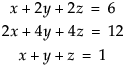
The GInverse() function accepts any matrix, including non-square ones, and uses singular-value decomposition to calculate the Moore-Penrose generalized inverse. The generalized inverse can be useful when inverting a matrix that is not full rank. Consider the following system of equations:
The Solve() function solves a system of linear equations. Solve() finds the vector x so that x = A-1b where A equals a square, nonsingular matrix and b is a vector. The matrix A and the vector b must have the same number of rows. Solve(A,b) is the same as Inverse(A)*b.
The Sweep() function inverts parts (or pivots) of a square matrix. If you sequence through all of the pivots, you are left with the matrix inverse. Normally the matrix must be positive definite (or negative definite) so that the diagonal pivots never go to zero. Sweep() does not check whether the matrix is positive definite. If the matrix is not positive definite, then it still works, as long as no zero pivot diagonals are encountered. If zero (or near-zero) pivot diagonals are encountered on a full sweep, then the result is a g2 generalized inverse if the zero pivot row and column are zeroed.

The syntax for Sweep() appears as follows:
|
•
|
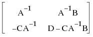
The submatrix in the A position becomes the inverse.
|
|
•
|
|
•
|
Sweep() is sequential and reversible:
|
•
|
A=Sweep(A,{i,j}) is the same as A=Sweep(Sweep(A,i),j). It is sequential.
|
|
•
|
A=Sweep(Sweep(A,i),i) restores A to its original values. It is reversible.
|
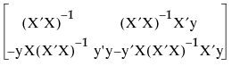
Then after sweeping through the indices of X’X, the result appears as follows:
|
•
|
the least squares estimates for the model Y = Xb + e in the upper right
|
The Sweep function is useful in computing the partial solutions needed for stepwise regression.
The index argument is a vector that lists the rows (or equivalently the columns) on which you want to sweep the matrix. For example, if E is a 4x4 matrix, to sweep on all four rows to get E-1 requires these commands:
Note: For a tutorial on Sweep(), and its relation to the Gauss-Jordan method of matrix inversion, see Goodnight, J.H. (1979) “A tutorial on the SWEEP operator.” The American Statistician, August 1979, Vol. 33, No. 3. pp. 149–58.
Sweep() is further demonstrated in the ANOVA Example.
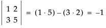
The Det() function returns the determinant of a square matrix. The determinant of a 2 × 2 matrix is the difference of the diagonal products, as demonstrated below. Determinants for n × n matrices are defined recursively as a weighted sum of determinants for (n - 1) × (n - 1) matrices. For a matrix to have an inverse, the determinant must be nonzero.
The Eigen() function performs eigenvalue decomposition of a symmetric matrix. Eigenvalue decompositions are used in many statistical techniques, most notably in principal components and canonical correlation, where the transformation associated with the largest eigenvalues are transformations that maximize variances.
Eigen() returns a list of matrices. The first matrix in the returned list is a column vector of eigenvalues; the second matrix contains eigenvectors as the columns.
For some n × n matrix A, eigenvalue decomposition finds all λ (lambda) and vectors x, so that the equation Ax = λx has a nonzero solution x. The λ’s are called eigenvalues, and the corresponding x vectors are called eigenvectors. This is equivalent to solving (A - λI)x = 0. You can reconstruct A from eigenvalues and eigenvectors by a statement like the following:
|
•
|
|
•
|
The Cholesky() function performs Cholesky decomposition. A positive semi-definite matrix A is re-expressed as the product of a nonsingular, lower-triangular matrix L and its transpose: L*L' = A.
Cholesky() is useful for reconstituting expressions into a more manageable form. For example, eigenvalues are available only for symmetric matrices in JMP, so the eigenvalues of the product AB could not be obtained directly. (Although A and B can be symmetric, the product is not symmetric.) However, you can usually rephrase the problem in terms of eigenvalues of L’BL where L is the Cholesky root of A, which has the same eigenvalues.
Another use of Cholesky() is in reordering matrices within Trace() expressions. Expressions such as Trace(A*B*A`) might involve huge operations counts if A has many rows. However, if B is small and can be factored into LL’ by Cholesky, then it can be reformulated to Trace(A*L*L`*A`). The resulting matrix is equal to Trace(L`A`*AL). This expression involves a much smaller number of operations, because it consists of only the sum of squares of the AL elements.
Use the function Chol Update() to update a Cholesky decomposition. If L is the Cholesky root of a n × n matrix A, then after using cholUpdate(L, C, V), L will be replaced with the Cholesky root of A+V*C*V'. C is an m × m symmetric matrix and V is an n × m matrix.
Instead of manual updating, use Chol Update() to update the Cholesky decomposition, as follows:
The SVD() function finds the singular value decomposition of a matrix. That is, for a matrix A, SVD() returns a list of three matrices U, M, and V, so that U*diag(M)*V`=A.
|
•
|
|
•
|
Singular value decomposition re-expresses A in the form USV’, where:
|
|
‒
|
U and V are matrices that contain orthogonal column vectors (perpendicular, statistically independent vectors)
|
|
‒
|
S is a n × n diagonal matrix containing the nonnegative square roots of the eigenvalues of A’A, the singular values of A.
|
The Ortho() function orthogonalizes the columns and then divides the vectors by their magnitudes to normalize them. This function uses the Gram-Schmidt method. The column vectors of orthogonal matrices are unit-length and are mutually perpendicular (their dot products are zero).
To verify that these vectors are orthogonal, multiply B by its transpose, which should yield the identity matrix.
By default, vectors are normalized, meaning that they are divided by their magnitudes, which scales them to have length 1. Include the option Scaled(0) to turn scaling off:
To create vectors whose elements sum to zero, include the Centered(1) option. This option is useful when constructing a matrix of contrasts.
The OrthoPoly() function returns orthogonal polynomials for a vector of indices. The polynomial order is specified as a function argument. Orthogonal polynomials can be useful for fitting polynomial models where some regression coefficients might be highly correlated.
The polynomial order must be less than the dimension of the vector. Use the Scaled(1) option to produce vectors of unit length, as described in Orthonormalization.
QR() factorization is useful for numerically stable matrix work. QR() returns a list of two matrices. The typical usage is as follows:
Q and R hold the results. For a m × n matrix, QR() creates an orthogonal m × m matrix Q and an upper triangular m × n matrix R, so that X = Q*R.
To add or drop one or more rows in an inverse of an M`M matrix, use the Inv Update(S, X, w) function. Updating inverse matrices is helpful in drop-1 influence diagnostics and also in candidate design evaluation.
|
•
|
The first argument, S, is the matrix to be updated.
|
|
•
|
The second argument, X, is the matrix of rows to be added or dropped.
|
|
•
|
Using the Inv Update(S, X, w) function is equivalent to calculating the following:
You can store your own operations in macros. See Macros in Programming Methods. Similarly, you can create custom matrix operations. For example, you can make your own matrix operation called Mag() to find the magnitude of a vector, as follows:
Similarly, you could create an operation called Normalize to divide a vector by its magnitude, as follows:
|
•
|
Y is a vector of responses
|
|
•
|
a is the intercept term
|
|
•
|
b is a vector of coefficients
|
|
•
|
X is a design matrix for the factor
|
|
•
|
e is an error term
|
Next, add a column of 1s to the design matrix for the intercept term. You can do this by concatenating J and Design Nom(), as follows:
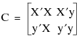
Now, to solve the normal equation, you need to construct a matrix M with partitions:

You can construct matrix M in one step by concatenating the pieces, as follows:
Now, sweep M over all the columns in X’X for the full fit model, and over the first column only for the intercept-only model:
|
•
|
You could modify this into a generalized ANOVA script by replacing some of the explicit values in the script with arguments. These results match those from the Fit Model platform. See ANOVA Report Within Fit Model.
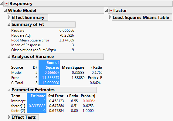
Construct the report in ANOVA Report Within Fit Model as follows:
|
3.
|