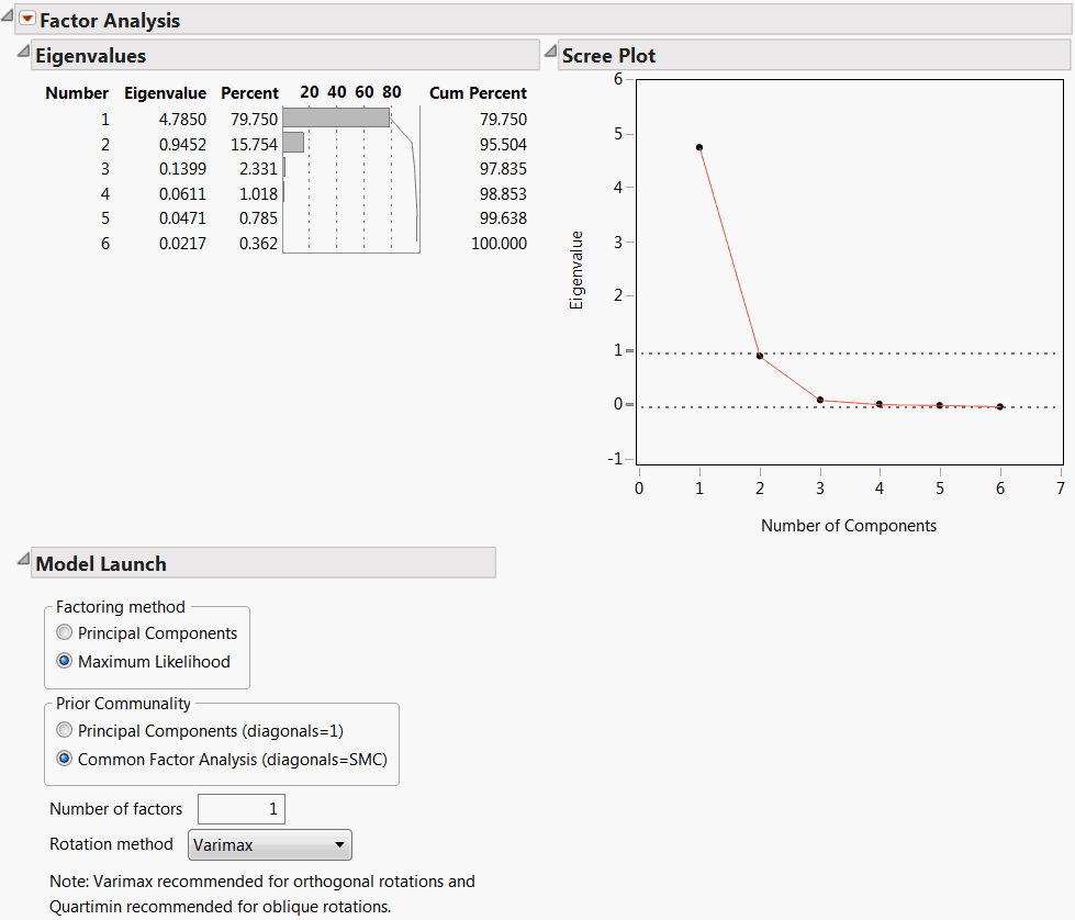
In the example shown in Factor Analysis Report, the Scree Plot begins to level out after the second eigenvalue. The Eigenvalues table indicates that the first eigenvalue accounts for 79.75% of the variation and the second eigenvalue accounts for 15.75%, for a total of 95.50% of the total variation. The third eigenvalue only explains 2.33% of the variation, and the contributions from the remaining eigenvalues are negligible. Although the Number of factors box is initially set to 1, this analysis suggests that extracting 2 factors is appropriate.
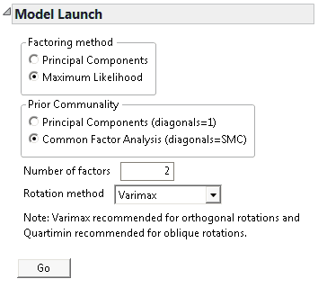
To configure the Factor Analysis model, use the Model Launch section at the bottom of the Factor Analysis Report (Model Launch).
|
1.
|
Factoring method - the method for extracting factors.
|
|
‒
|
The Principal Components method is a computationally efficient method, but it does not allow for hypothesis testing.
|
|
‒
|
The Maximum Likelihood method has desirable properties and allows you to test hypotheses about the number of common factors.
|
Note: The Maximum Likelihood method requires a positive definite correlation matrix. If your correlation matrix is not positive definite, select the Principal Components method.
|
2.
|
Prior Communality - the method for estimating the proportion of variance contributed by common factors for each variable.
|
|
‒
|
Principal Components (diagonals = 1) sets all communalities equal to 1, indicating that 100% of each variable’s variance is shared with the other variables. Using this option with Factoring Method set to Principal Components results in principal component analysis.
|
|
‒
|
Common Factor Analysis (diagonals = SMC) sets the communalities equal to squared multiple correlation (SMC) coefficients. For a given variable, the SMC is the RSquare for a regression of that variable on all other variables.
|
|
3.
|
The Number of factors (or principal components) determined by eigenvalues greater than or equal to 1.0 or from the scree plot where the graph begins to level out.
|
Note: Alternatively, the Kaiser criterion retains those factors with eigenvalues greater than 1.0. In our example, only factor 1 would be retained for analysis.
|
4.
|
The Rotation method to align the factor directions with the original variables for ease of interpretation. The default value is Varimax. See Rotation Methods for a description of the available selections.
|
|
5.
|
Click Go to generate the Factor Analysis report.
|
Depending on the selected Variance Scaling, the appropriate factor analysis results appear. See Factor Analysis Model Fit Options for details about the contents of the report. The Factor Analysis on Correlations and Factor Analysis on Unscales reports show the same information.
Orthogonal Rotation Methods lists the available orthogonal (that is, uncorrelated) rotation methods.
|
Note: The default p value is 1 unless specified otherwise in the GAMMA = option. For additional information about orthomax weight, see the SAS documentation, “Simplicity Functions for Rotations.”
|
|
Oblique Rotation Methods lists the available oblique (that is, correlated) rotation methods.
|
ROTATE=OBLIMIN, where the default p value is zero, unless specified otherwise in the TAU= option.
|
|