The way the x-variables (factors) are modeled to predict an expected value or probability is the subject of the factor side of the model.
The factors enter the prediction equation as a linear combination of x values and the parameters to be estimated. For a continuous response model, where i indexes the observations and j indexes the parameters, the assumed model for a typical observation, yi, is written
yi is the response
xij are functions of the data
ei is an unobservable realization of the random error
bj are unknown parameters to be estimated.
The way the x’s in the linear model are formed from the factor terms is different for each modeling type. The linear model x’s can also be complex effects such as interactions or nested effects. Complex effects are discussed in detail later.
Continuous factors are placed directly into the design matrix as regressors. If a column is a linear function of other columns, then the parameter for this column is marked zeroed or nonestimable. Continuous factors are centered by their mean when they are crossed with other factors (interactions and polynomial terms). Centering is suppressed if the factor has a Column Property of Mixture or Coding, or if the centered polynomials option is turned off when specifying the model. If there is a coding column property, the factor is coded before fitting.
|
1´
|
||
|
|
||
|
|
Using the JMP Fit Model command and requesting a factorial model for columns A and B produces the following design matrix. Note that A13 in this matrix is A1–A3 in the previous matrix. However, A13B13 is A13*B13 in the current matrix.
|
|
|
|
|
|
|
|
|
|
|
|
|
|
Least squares means are the predicted values corresponding to some combination of levels, after setting all the other factors to some neutral value. The neutral value for direct continuous regressors is defined as the sample mean. The neutral value for an effect with uninvolved nominal factors is defined as the average effect taken over the levels (which happens to result in all zeroes in our coding). Ordinal factors use a different neutral value in Ordinal Least Squares Means. The least squares means might not be estimable, and if not, they are marked nonestimable. JMP’s least squares means agree with GLM’s (Goodnight and Harvey 1978) in all cases except when a weight is used, where JMP uses a weighted mean and GLM uses an unweighted mean for its neutral values.
|
•
|
JMP implements the effective hypothesis tests described by Hocking (1985, 80–89, 163–166), although JMP uses structural rather than cell-means parameterization. Effective hypothesis tests start with the hypothesis desired for the effect and include “as much as possible” of that test. Of course, if there are containing effects with missing cells, then this test will have to drop part of the hypothesis because the complete hypothesis would not be estimable. The effective hypothesis drops as little of the complete hypothesis as possible.
|
With linear dependencies, a least squares solution for the parameters might not be unique and some tests of hypotheses cannot be tested. The strategy chosen for JMP is to set parameter estimates to zero in sequence as their design columns are found to be linearly dependent on previous effects in the model. A special column in the report shows what parameter estimates are zeroed and which parameter estimates are estimable. A separate singularities report shows what the linear dependencies are.
|
|
|
|
|
|
|
|
|
|
|

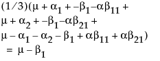
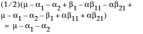
Note that this shows that a test on the β1 parameter is equivalent to testing that the least squares means are the same. But because β1 is not estimable, the test is not testable, meaning there are no degrees of freedom for it.
|
a1
|
||
|
a2
|
||
|
b1
|
||
|
ab11
|
||
|
ab21
|
|
4.
|
The tests are whole marginal tests, meaning they always go completely across other effects in interactions.
|
Comparison of GLM and JMP Hypotheses, shows the test of the main effect A in terms of the GLM parameters. The first set of columns is the test done by JMP. The second set of columns is the test done by GLM Type IV. The third set of columns is the test equivalent to that by JMP; it is the first two columns that have been multiplied by a matrix:
noting that μ is the expected response at A = 1, μ + α2 is the expected response at A = 2, and μ + α2 + α3 is the expected response at A = 3. Thus, α2 estimates the effect moving from A = 1 to A = 2 and α3 estimates the effect moving from A = 2 to A = 3.
To see what the parameters mean, examine this table of the expected cell means in terms of the parameters, where μ is the intercept, α2 is the parameter for level A2, and so forth.
|
|
|
|
|
|
|
|
|
|
|
|
|
|
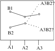
Note that the main effect test for A is really testing the A levels holding B at the first level. Similarly, the main effect test for B is testing across the top row for the various levels of B holding A at the first level. This is the appropriate test for an experiment where the two factors are both doses of different treatments. The main question is the efficacy of each treatment by itself, with fewer points devoted to looking for drug interactions when doses of both drugs are applied. In some cases it may even be dangerous to apply large doses of each drug.
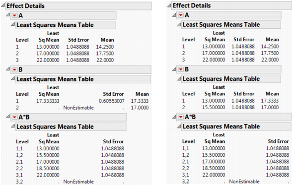
The example is the same as above, with two observations per cell except that the A3B2 cell has no data. You can now compare the results when the factors are coded nominally with results when they are coded ordinally. The model fit is the same, as seen in Summary Information for Nominal Fits (Left) and Ordinal Fits (Right).
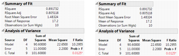
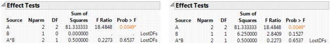
The effect tests lose degrees of freedom for nominal. In the case of B, there is no test. For ordinal, there is no loss because there is no missing cell for the base first level.
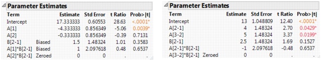
The least squares means are also different. The nominal LSMs are not all estimable, but the ordinal LSMs are. You can verify the values by looking at the cell means. Note that the A*B LSMs are the same for the two. Least Squares Means for Nominal Fits (Left) and Ordinal Fits (Right) shows least squares means for an nominal and ordinal fits.