Create a Nonlinear Design with No Prior Data
This example shows how to create a design when you have not yet collected data, but have a guess for the unknown parameters. In this example, you model the fractional yield (Observed Yield) of an intermediate product in a chemical reaction. The fractional yield is a function of reaction time and temperature. See Box and Draper (1987).
Create the Design
1. Select Help > Sample Data Library and open Design Experiment/Reaction Kinetics Start.jmp.
Notice the following:
– The data table contains no rows because no data have been collected.
– The columns for the predictors, Reaction Temperature and Reaction Time, have the Coding, Design Role, and Factor Changes properties. To see these properties, click ![]() in the Columns panel. They tell JMP how to treat these predictors when constructing a design. For information about how to save these column properties, see Column Properties.
in the Columns panel. They tell JMP how to treat these predictors when constructing a design. For information about how to save these column properties, see Column Properties.
– The Observed Yield column will contain response data obtained by running the experiment.
– The Yield Model column contains the formula that relates the predictors to the response, Observed Yield. Click  in the Columns panel to see the formula. The formula is nonlinear in the parameters t1 and t3.
2. Select DOE > Special Purpose > Nonlinear Design.
3. Select Observed Yield and click Y, Response.
4. Select Yield Model and click X, Predictor Formula.
5. Click OK.
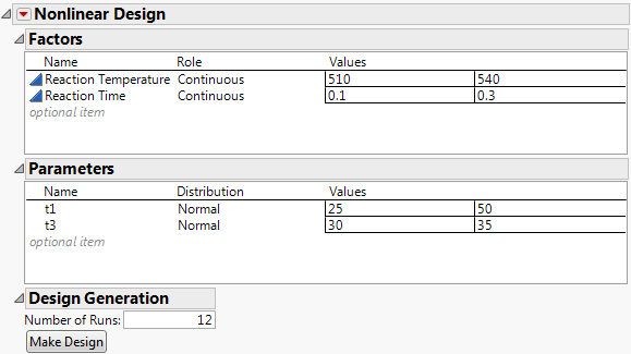
In this example, the values 510 and 540 for Reaction Temperature and 0.1 and 0.3 for Reaction Time were specified using the Coding column property. Alternatively, you can specify a reasonable range of values directly in the Factors outline.
6. Change the values of the parameter t1 to 25 and 50, and t3 to 30 and 35.
These new values represent a reasonable range of parameter values for the experimental situation. The default values were constructed based on the initial parameter values that were specified in the definition of the prediction formula. For information about constructing formulas, see Formula Editor in Using JMP.
Notice that the prior distribution, shown under Distribution, for each of t1 and t3 is set to Normal by default.
7. Change the number of runs to 12 in the Design Generation panel.
Figure 23.2 Completed Outlines for Reaction Kinetics Experiment
8. Click Make Design.
9. Click Make Table.
Figure 23.3 Design Table
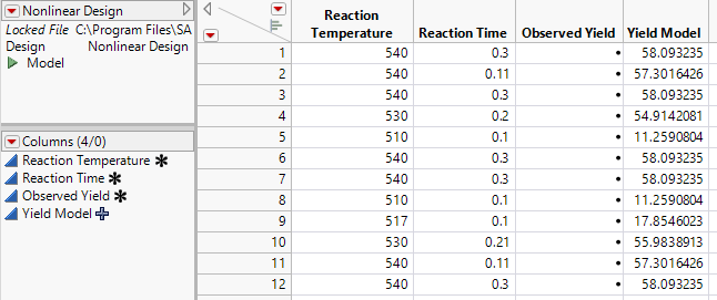
Your design should be similar to the one shown in Figure 23.3. The runs might be in a different order, and the values for Reaction Temperature and Reaction Time, and consequently those computed for Yield Model, can be slightly different. Notice that values appear in the Yield Model column because the column contains the formula for the model. Also notice that the table contains a Model script that you can use to fit a nonlinear model to your observations.
Now that you have created your design table, run your experiment, and record the responses in the Observed Yield column. The data table Reaction Kinetics.jmp, found in the Design Experiment folder contains observed results for the design.
Explore the Design
Before analyzing your results, construct a plot to see the design settings.
1. Select Help > Sample Data Library and open Design Experiment/Reaction Kinetics.jmp.
1. Select Graph > Graph Builder.
2. Drag and drop Reaction Temperature into the Y zone.
3. Drag and drop Reaction Time into the X zone.
4. Click the second icon above the graph to deselect the Smoother.
Figure 23.4 Design Settings
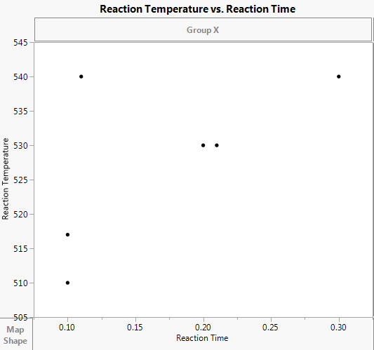
Notice that the points are located in three areas. There are no points at low temperature and high time (the lower right corner of the graph). Unlike orthogonal designs, nonlinear designs do not necessarily place design points at the corners of the design region. In this example, design points at low temperature and high time would be inefficient.
To see the density of design points in the remaining three corners, use the Contour tool.
5. Click ![]() to turn on the Contour tool.
to turn on the Contour tool.
6. Click Done.
Figure 23.5 Design Settings with Density Contours
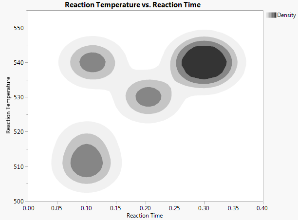
Notice that there are comparatively few points at low time and high temperature. From the design table, you can see that there are only two such points. Because of the model and the parameter specifications, the optimal design places more design points at high time and high temperature.
Analyze the Results
Now that you visually explored your design, analyze your results.
Note: Rather than conduct step 1 through step 4, you can run the Model script.
1. Select Analyze > Specialized Modeling > Nonlinear.
2. Select Observed Yield and click Y, Response.
3. Select Yield Model and click X, Predictor Formula.
Notice that the model appears in the Options for fitting custom formulas panel.
4. Click OK.
5. Click Go in the Control Panel.
The iterative search for a solution proceeds until one of the Stop Limit values is reached. Then, the Solution and Correlation of Estimates reports appear.
6. Click the Nonlinear Fit red triangle and select Profilers > Profiler.
7. To maximize the yield, click the Prediction Profiler red triangle and select Optimization and Desirability > Maximize Desirability.
Figure 23.6 Time and Temperature Settings for Maximum Yield
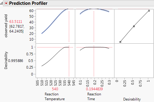
The estimated maximum yield is approximately 63.5% at a reaction temperature of 540 degrees Kelvin and a reaction time of 0.1945 minutes.