Example Using Mixed Model

In a study of wheat yield, 10 varieties of wheat are randomly selected from the population of varieties of hard red winter wheat adapted to dry climate conditions. These are randomly assigned to six one-acre plots of land. The preplanting moisture content of the plots could influence the germination rate and hence the eventual yield of the plots. Thus, the amount of preplanting moisture in the top 36 inches of soil is determined for each plot. You are interested in determining if the moisture content affects yield.

Because the varieties are randomly selected, the regression model for each variety is a random model selected from the population of variety models. The intercept and slope are random for each variety and might be correlated. The random coefficients are centered at the fixed effects. The fixed effects are the population intercept and the slope, which are the expected values of the population of the intercepts and slopes of the varieties. This example is taken from Littell et al. (2006, p. 320).

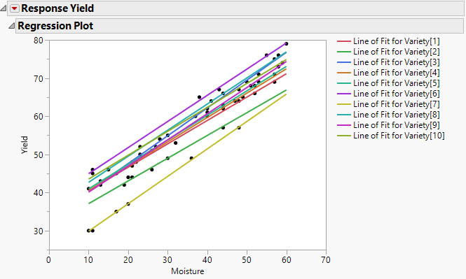
Fitting the model using REML in the Standard Least Squares personality lets you view the variation in intercepts and slopes (Figure 8.2). Note that the slopes do not have much variability, but the intercepts have quite a bit. The intercept and slope might be negatively correlated; varieties with lower intercepts seem to have higher slopes.

Figure 8.2 Standard Least Squares Regression 

To model the correlation between the intercept and the slope, use the Mixed Models personality. You are interested in determining the population regression equation as well as variety-specific equations.

1. Select Help > Sample Data Library and open Wheat.jmp.

2. Select Analyze > Fit Model.

3. Select Yield and click Y.

When you add this column as Y, the fitting Personality becomes Standard Least Squares.

4. Select Mixed Model from the Personality list. Alternatively, you can select the Mixed Model personality first, and then click Y to add Yield.

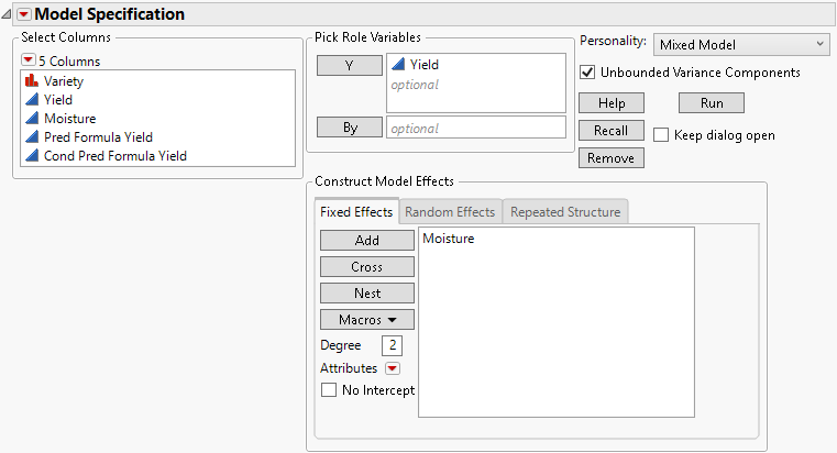
5. Select Moisture and click Add on the Fixed Effects tab.

Figure 8.3 Completed Fit Model Launch Window Showing Fixed Effects 

6. Select the Random Effects tab.

7. Select Moisture and click Add.

8. Select Variety from the Select Columns list, select Moisture from the Random Effects tab, and then click Nest Random Coefficients.

Figure 8.4 Completed Fit Model Launch Window Showing Random Effects Tab 

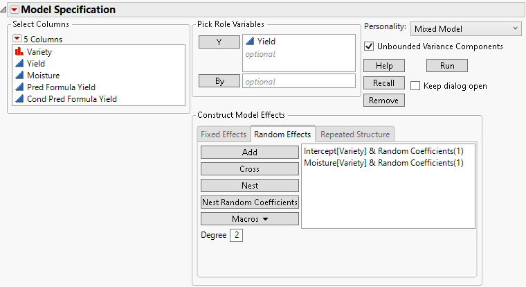
Random effects are grouped by variety, and the intercept is included as a random component.

9. Click Run.

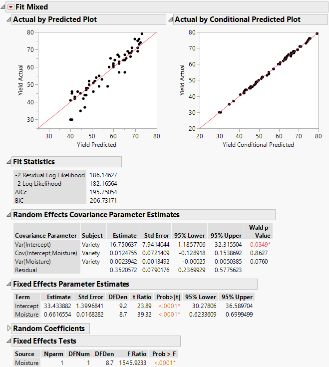
The Fit Mixed report is shown in Figure 8.5. Note that some of the constituent reports are closed because of space considerations. The Actual by Predicted plot shows no discrepancy in terms of model fit and underlying assumptions.

Because there are no apparent problems with the model fit, you can now interpret the statistical tests and obtain the regression equation. The effect of moisture upon yield is significant, as shown in the Fixed Effects Tests report. The estimates given in the Fixed Effects Parameter Estimates indicate that the estimated population regression equation is as follows:

Yield = 33.43 + 0.66 * Moisture

The Random Effects Covariance Parameter Estimates report gives estimates of the variance of the varieties’ intercepts, Var(Intercept), and slopes, Var(Moisture), and their covariance, Cov(Moisture, Intercept). In this case, the intercept and slope are not significantly correlated, because the confidence interval for the estimate includes zero. The report also gives an estimate of the residual variance.

Figure 8.5 Fit Mixed Report 

Although you have an estimate of the population regression equation, you are also interested in Variety 2’s estimated yield.

10. Open the Random Coefficients report to see the estimates of the variety effects for Intercept and Moisture. These coefficients estimate how each variety differs from the population.

Figure 8.6 Random Coefficients Report 

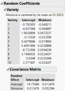
In the Model Specification window, the Center Polynomials option is selected by default. Because of this, the Moisture effect is centered at its mean of 35.583, as stated in the note at the top of the Variety report. From the Fixed Effects Parameter Estimates and Random Coefficients reports, you obtain the following prediction equation for Variety 2:

Yield = 33.433 + 0.662 * Moisture – 4.658 – 0.067 * (Moisture – 35.583)

Yield = 31.159 + 0.595 * Moisture

Variety 2 starts with a lower yield than the population average and increases with Moisture at a slower rate than the population average.