Example Using the Reliability Forecast Platform
You have data on seven months of production and returns. You need to use this information to forecast the total number of units that will be returned for repair through February 2011.The product has a 12-month contract.
1. Select Help > Sample Data Library and open Reliability/Small Production.jmp.
2. Select Analyze > Reliability and Survival > Reliability Forecast.
3. On the Nevada Format tab, select Sold Quantity and click Production Count.
4. Select Sold Month and click Timestamp role.
5. Select the other columns and click Failure Count.
6. Click OK.
Figure 9.2 Observed Data Report
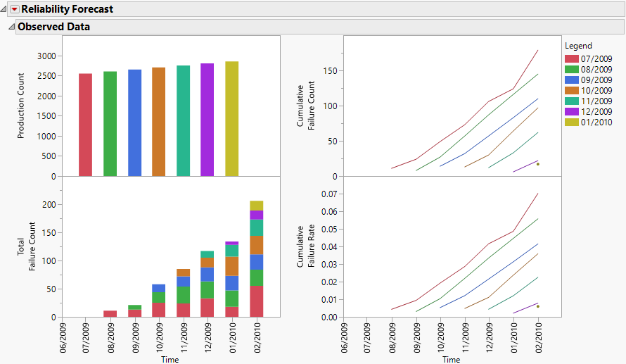
On the bottom left, the Observed Data report shows bar charts of previous failures. Cumulative failures are shown on the line graphs. Note that production levels are fairly consistent. As production accumulates over time, more units are at risk of failure, so the cumulative failure rate gradually rises. The consistent production levels also result in similar cumulative failure rates and counts.
7. Click the Life Distribution disclosure icon.
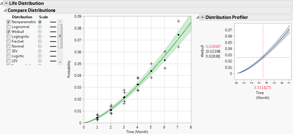
JMP fits production and failure data to a Weibull distribution using the Life Distribution platform (Figure 9.3). JMP then uses the fitted Weibull distribution to forecast returns for the next five months (Figure 9.4).
Figure 9.3 Life Distribution Report
The Forecast report shows previous production on the left graph (Figure 9.4). On the right graph, you see that the number of previous failures increased steadily over time.
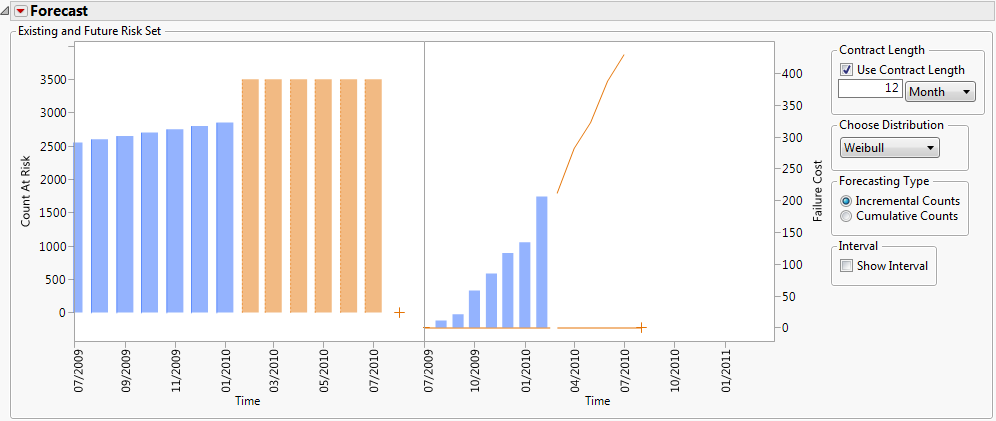
Figure 9.4 Forecast Report
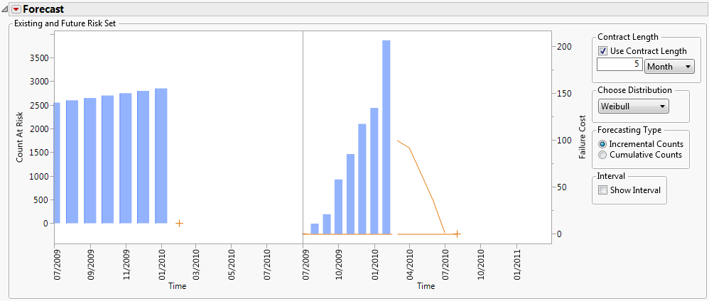
8. In the Forecast report, type 12 for the Contract Length. This is the contract length.
9. On the left Forecast graph, drag the animated hotspot over to July 2010 and upward to approximately 3500.
Orange bars appear on the left graph to represent future production. The monthly returned failures in the right graph increase gradually through August 2010.
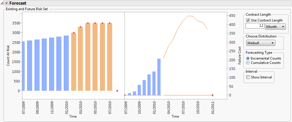
Figure 9.5 Production and Failure Estimates
10. Drag the February 2010 hotspot to approximately 3000 and then drag the March 2010 hotspot to approximately 3300.
11. On the right graph, drag the right hotspot to February 2011.
JMP estimates that the number of returns will gradually increase through August 2010 and decrease by February 2011.
Figure 9.6 Future Production Counts and Forecasted Failures