Forecast Report
The Forecast report provides interactive graphs that help you forecast failures. By dragging hotspots, you can add anticipated production counts and see how they affect the forecast.
Adjusting Risk Sets
Future Production
On the left graph, the blue bars represent previous production counts. To add anticipated production, follow these steps:
1. Drag a hotspot to the right to add one or more production periods.
The orange bars represent future production.
Figure 9.11 Add Production Periods
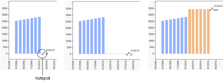
2. Drag each bar upward or downward to change the production count for each period.
Figure 9.12 Adjust Production Counts
Tip: To adjust future production counts, click the Forecast red triangle and select Spreadsheet Configuration of Risk Sets. See Spreadsheet Configuration of Risk Sets.
Existing Production
Right-click a blue bar and select Exclude to remove that risk set from the forecast results. You can then right-click and select Include to return that data to the risk set.
Tip: To adjust existing production counts, click the Forecast red triangle and select Spreadsheet Configuration of Risk Sets. See Spreadsheet Configuration of Risk Sets.
Forecasting Failures
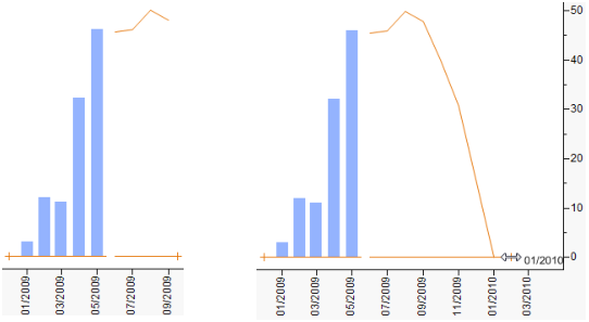
When you adjust production in the left graph, the right graph is updated to estimate future failures (Figure 9.13). Dragging a hotspot lets you change the forecast period. The orange line then shortens or lengthens to show the estimated failure counts.
Figure 9.13 Adjust the Forecast Period
Defining Risk Sets with Time to Event Data
You can obtain forecasts for arbitrary risk sets using the Time to Event Format tab. In the launch window’s Time to Event Format tab, the Life Time Unit must be selected as Numeric and the Forecast Start Time must be set to zero. Enter appropriate columns for Time to Event, Censor, Freq, and Group ID.
The plot on the left provides locations for bars representing existing production. Drag the hotspot at 0 to the left to create existing risk sets. Drag the hotspot at 1 to the right to create future production risk sets.
Existing and future risk sets can also be specified using the Spreadsheet Configuration of Risk Sets option. Values for the existing risk set for time to event data must be entered in the Future Risk area using negative time values. See Spreadsheet Configuration of Risk Sets.
Forecast Graph Options
As you work with the graphs, you can change the contract length, distribution type, and other options to explore your data further.
• To forecast failures for a different contract period, enter the number next to Use Contract Length. Change the time unit if necessary.
• To change the distribution fit, select a distribution from the Choose Distribution list. The distribution is then fit to the future graph of future risk. The distribution fit appears on the Life Distribution report plot, and a new profiler is added. Note that changing the distribution fit in the Life Distribution report does not change the fit on the Forecast graph.
• If you are more interested in the total number of failures over time, select Cumulative Counts. Otherwise, JMP shows failures incrementally, which might make trends easier to identify.
• To show confidence limits for the anticipated number of failures, select Show Interval.
Forecast Report Options
The Forecast red triangle menu contains the following options:
Animation
Controls the flashing of the hotspots. You can also right-click a blue bar in the existing risk set and select or deselect Animation.
Interactive Configuration of Risk Sets
Determines whether you can drag hotspots in the graphs.
Spreadsheet Configuration of Risk Sets
Lets you specify production counts and periods (rather than adding them to the interactive graphs). You can also exclude production periods from the analysis.
– To remove an existing time period from analysis, highlight the period in the Existing Risk area, click, and then select Exclude. Or select Include to return the period to the forecast.
– To edit production, double-click in the appropriate Future Risk field and enter the new values.
– To add a production period to the forecast, right-click in the Future Risk area and select one of the Append options. (Append Rows adds one row; Append N Rows lets you specify the number of rows.)
As you change these values, the graphs update accordingly.
Note: If you launched the platform using the Time to Event Format tab, values for the existing risk set must be entered in the Future Risk area using negative time values.
Import Future Risk Set
Lets you import future production data from another open data table. The new predictions then appear on the future risk graph. The imported data must have a column for timestamps and for quantities.
Show Interval
Shows or hides confidence limits on the graph. This option works the same as selecting Show Interval next to the graphs.
After you select Show Interval, the Forecast Interval Type option appears on the menu. Select one of the following interval types:
Plugin Interval
Considers only forecasting errors given a fixed distribution.
Prediction Interval
Considers forecasting errors when a distribution is estimated with estimation errors (for example, with a non-fixed distribution).
If the Prediction interval is selected, the Prediction Interval Settings option appears in the menu. Approximate intervals are initially shown on the graph. Select Monte Carlo Sample Size or Random Seed to specify those values instead. To use the system clock, enter a missing number.
Use Contract Length
Determines whether the specified contract length is considered in the forecast. This option works the same as selecting Use Contract Length next to the graphs.
Use Failure Cost
Shows failure cost instead of the failure count on the future risk graph.
After you select Use Failure Cost, the Set Failure Cost option appears on the menu. This option enables you to set a cost for each failure. If you specified a Group variable in the launch window, the Set Failure Cost window enables you to specify separate costs for failures in each group.
Save Forecast Data Table
Saves the cumulative and incremental number of returns in a new data table, along with the variables that you selected in the launch window. For grouped analyses, table names include the group ID and the word “Aggregated”. And existing returns are included in the aggregated data tables.