Launch the Partial Least Squares Platform
There are two ways to launch the Partial Least Squares platform:
• Select Analyze > Multivariate Methods > Partial Least Squares.
•  Select Analyze > Fit Model and select Partial Least Squares from the Personality menu. This approach enables you to do the following:
– Enter categorical variables as Ys or Xs. Conduct PLS-DA by entering categorical Ys.
– Add interaction and polynomial terms to your model.
– Use the Standardize X option to construct higher-order terms using centered and scaled columns.
– Save your model specification script.
Some features on the Fit Model launch window are not applicable for the Partial Least Squares personality:
• Weight, Nest, Attributes, Transform, and No Intercept.
Tip: You can transform a variable by right-clicking it in the Select Columns box and selecting a Transform option.
• The following Macros: Mixture Response Surface, and Scheffé Cubic.
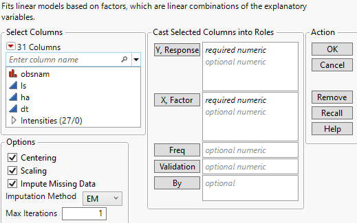
Figure 6.6 JMP Pro Partial Least Squares Launch Window (Imputation Method EM Selected)
For more information about the options in the Select Columns red triangle menu, see Column Filter Menu in Using JMP.
The Partial Least Squares launch window contains the following options:
Y, Response
Enter numeric response columns. If you enter multiple columns, they are modeled jointly.
 In JMP Pro, you can enter nominal response columns in the Fit Model launch window to conduct PLS-DA. See PLS Discriminant Analysis (PLS-DA).
X, Factor
Enter the predictor columns. The Partial Least Squares launch window allows only numeric predictors.
 In JMP Pro, you can enter nominal and ordinal model effects in the Fit Model launch window. Ordinal effects are treated as nominal.
Freq
If your data are summarized, enter the column whose values contain counts for each row.
 Validation
Enter an optional validation column. A validation column must contain only consecutive integer values. Note the following:
– If the validation column has two levels, the smaller value defines the training set and the larger value defines the validation set.
– If the validation column has three levels, the values define the training, validation, and test sets in order of increasing size.
– If the validation column has more than three levels, then KFold Cross Validation is used. For information about other validation options, see Validation Method.
Note: If you click the Validation button with no columns selected in the Select Columns list, you can add a validation column to your data table. For more information about the Make Validation Column utility, see Basic Analysis.
By
Enter a column that creates a report consisting of separate analyses for each level of the variable. If more than one By variable is assigned, a separate analysis is produced for each possible combination of the levels of the By variables.
Centering
Centers all Y variables and model effects by subtracting the mean from each column. See Centering and Scaling.
Scaling
Scales all Y variables and model effects by dividing each column by its standard deviation. See Centering and Scaling.
 Standardize X
(Available only in the Fit Model launch window.) Centers and scales all columns that are used in the construction of model effects. If this option is not selected, higher-order effects are constructed using the original data table columns. Then each higher-order effect is centered or scaled, based on the selected Centering and Scaling options. Note that Standardize X does not center or scale Y variables. See Standardize X.
 Impute Missing Data
Replaces missing data values in Ys or Xs with nonmissing values. Select the appropriate method from the Imputation Method list.
If Impute Missing Data is not selected, rows that are missing observations on any X variable are excluded from the analysis and no predictions are computed for these rows. Rows with no missing observations on X variables but with missing observations on Y variables are also excluded from the analysis, but predictions are computed.
 Imputation Method
(Appears only when Impute Missing Data is selected.) Select from the following imputation methods:
Mean
For each model effect or response column, replaces the missing value with the mean of the nonmissing values.
EM
Uses an iterative Expectation-Maximization (EM) approach to impute missing values. On the first iteration, the specified model is fit to the data with missing values for an effect or response replaced by their means. Predicted values from the model for Y and the model for X are used to impute the missing values. For subsequent iterations, the missing values are replaced by their predicted values, given the conditional distribution using the current estimates.
For the purpose of imputation, polynomial terms are treated as separate predictors. When a polynomial term is specified, that term is calculated from the original data, or, if Standardize X is checked, from the standardized column values. If a row has a missing value for a column involved in the definition of the polynomial term, then that entry is missing for the polynomial term. Imputation is conducted using polynomial terms defined in this way.
For more information about the EM approach, see Nelson, Taylor, and MacGregor (1996).
 Max Iterations
(Appears only when EM is selected as the Imputation Method.) Enables you to set the maximum number of iterations used by the algorithm. The algorithm terminates if the maximum difference between the current and previous estimates of missing values is bounded by 10-8.
After completing the launch window and clicking OK, the Model Launch control panel appears. See Model Launch Control Panel.