Model Selection and Deviance

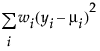
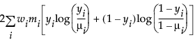
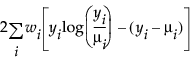
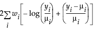
An important aspect of generalized linear modeling is the selection of explanatory variables in the model. Changes in goodness-of-fit statistics are often used to evaluate the contribution of subsets of explanatory variables to a particular model. The deviance is defined to be twice the difference between the maximum attainable log-likelihood and the log-likelihood at the maximum likelihood estimates of the regression parameters. The deviance is often used as a measure of goodness of fit. The maximum attainable log-likelihood is achieved with a model that has a parameter for every observation. Table 12.4 lists the deviance formula for each of the available distributions for the response variable.

The Pearson chi-square statistic is defined as follows:

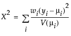
where

yi is the ith response

μi is the corresponding predicted mean

V(μi) is the variance function

wi is a known weight for the ith observation

Note: If no weight is specified, wi = 1 for all observations.

One strategy for variable selection is to fit a sequence of models. You start with a simple model that contains only an intercept term, and then include one additional explanatory variable in each successive model. You can measure the importance of the additional explanatory variable by the difference in deviance or fitted log-likelihood values between successive models. Asymptotic tests enable you to assess the statistical significance of the additional term.

When the distribution is non-normal, a normal critical value is used instead of a t-distribution critical value in inverse prediction.

Residual Formulas

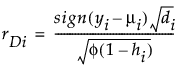
Deviance

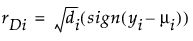
Studentized Deviance

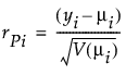
Pearson

Studentized Pearson

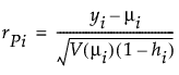
where

(yi – μi) is the raw residual

sign(yi – μi) is 1 if (yi – μi) is positive and -1 if (yi – μi) is negative

di is the contribution to the total deviance from observation i

φ is the dispersion parameter

V(μi) is the variance function

hi is the ith diagonal element of the matrix We(1/2)X(X'WeX)-1X'We(1/2), where We is the weight matrix used in computing the expected information matrix.

For more information about residuals and generalized linear models, see the GENMOD Procedure chapter in the SAS/STAT 14.3 User’s Guide (SAS Institute Inc. 2017, ch. 46).