One-Way Analysis of Variance Example
In a one-way analysis of variance, a different mean is fit to each of the different groups, as identified by a nominal variable. To specify the model for JMP, select a continuous response column and a nominal effect column. This example uses the data in Drug.jmp.
1. Select Help > Sample Data Library and open Drug.jmp.
2. Select Analyze > Fit Model.
3. Select y and click Y.
4. Select Drug and click Add.
5. Click Run.
In this example, Drug has three levels, a, d, and f. The standard least squares fitting method translates this specification into a linear model as follows: The nominal variables define a sequence of indicator variables, which assume only the values 1, 0, and –1. The linear model is written as follows:
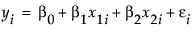
where:
– yi is the observed response for the ith observation
– x1i is the value of the first indicator variable for the ith observation
– x2i is the value of the second indicator variable for the ith observation
– β0, β1, and β2 are parameters for the intercept, the first indicator variable, and the second indicator variable, respectively
– εi are the independent and normally distributed error terms
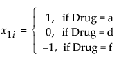
The first indicator variable, x1, is defined as follows. Note that Drug = a contributes a value 1, Drug = d contributes a value 0, and Drug = f contributes a value –1 to the indicator variable:
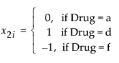
The second indicator variable, x2, is given the following values:
The estimates of the means for the three levels in terms of this parameterization are as follows:


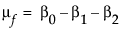
Solving for βi yields the following:
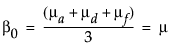 (the average over levels)


Therefore, if regressor variables are coded as indicators for each level minus the indicator for the last level, then the parameter for a level is interpreted as the difference between that level’s response and the average response across all levels. See the appendix Statistical Details for additional information about the interpretation of the parameters for nominal factors.
Figure 4.1 shows the Leverage Plot and the LS Means Table for the Drug effect. Figure 4.2 shows the Parameter Estimates and the Effect Tests reports for the one-way analysis of the drug data.
Figure 4.1 Leverage Plot and LS Means Table for Drug
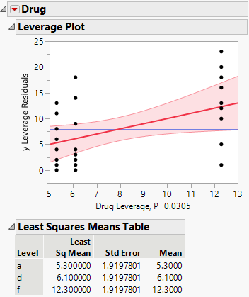
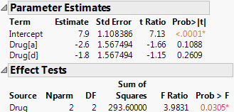
Figure 4.2 Parameter Estimates and Effect Tests for Drug.jmp
The Drug effect can be studied in more detail by using a contrast of the least squares means, as follows:
1. Click the Drug red triangle and select LSMeans Contrast.
2. Click the + boxes for drugs a and d, and the - box for drug f to define the contrast that compares the average of drugs a and d to f (shown in Figure 4.3).
3. Click Done.
Figure 4.3 Contrast Example for the Drug Experiment
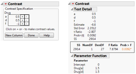
The Contrast report shows that the LSMean for drug f is significantly different from the average of the LSMeans of the other two drugs.