Specify Design Details
Specify the factor levels, details of the prior distribution, the time range and probability of interest, the length of the test, and the number of units to be tested.
Figure 22.18 Distribution Details
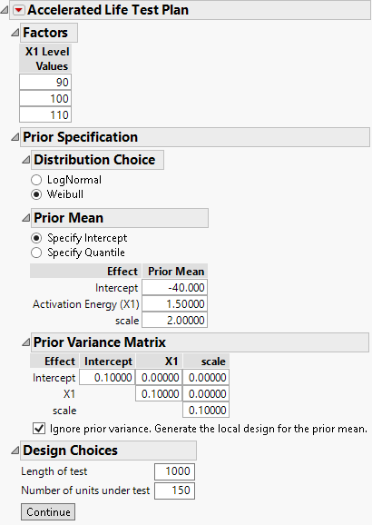
Factors
Enter the levels for the acceleration factors. By default, the levels are evenly spaced between the low and high test conditions.
Distribution Choice
Select a life distribution (Weibull or LogNormal) for each acceleration factor. See Statistical Details for the ALT Design Platform.
Prior Mean
Enter prior estimates of the acceleration model parameters. The prior estimates are hyperparameters in a Bayesian prior distribution. The Prior Mean values can be a best guess based on subject matter knowledge or they can be based on a previous study.
When there is only one acceleration factor, there is a choice to specify the intercept or the quantile.
Specify Intercept
Enter the priors for the model parameters including the intercept.
Specify Quantile
Enter the priors for the acceleration factor, the expected failure proportion at a given time and value for the acceleration factor. This information is used to calculate the intercept.
Prior Variance Matrix
Enter values for the variances and covariances of the prior distribution for the acceleration model parameters. These variances and covariances reflect uncertainty relative to the prior estimates of the acceleration model parameters. Large variances indicate greater uncertainty.
Ignore prior variance
Select this option to ignore the prior variances and covariances for the prior distribution. When these variances and covariances are ignored, the design is created by treating the values entered under Prior Mean as the true parameter values. This design is close to optimal if the prior mean parameters are close to the true values. However, this design is not robust to misspecification of the parameter estimates. If you are unsure about your prior estimates, use the Prior Variance Matrix to reflect your uncertainty.
Diagnostic Choices
The choices available depend on the design optimality criteria. For a D-optimal design there are no diagnostic choices.
Time range of interest
(Available only for a failure probability optimal design.) Specify the time interval over which you want to estimate the fraction of the population that is failing. Enter the lower value in the left box and the upper value in the right box. If you are interested in a specific time point, enter that value in both boxes.
Probability of interest
(Available only for a quantile estimate optimal design.) Specify the failure fraction for which you want an estimate of time. For example, if you want to estimate the time at which 10% of the units fail, then enter 0.10.
Design Choices
Specify values relating to the length of the test, inspection intervals, and the number of units being tested. Enter values for the following:
Length of test
(Available only for Continuous Monitoring.) Specify the length of time during which units are on test. When you make the design table, record each unit’s failure time or whether it was right censored.
Inspection Times
(Available only for Monitoring at Intervals.) Specify the times at which inspections are conducted. When you make the design table, these times are used to construct Start Time and End Time columns. The number of units failing in each interval is recorded.
Number of units under test
The number of units in the experiment.
– If you are designing an initial experiment, enter the number of units that you plan to test.
– If you are augmenting a previous experiment, enter the number of units tested in the previous experiment plus the number of units for the next experiment.