Structured Query Language (SQL): A Reference
The following sections are a brief introduction to SQL. They give you insight to the power of queries, and they are not meant to be a comprehensive reference.
Use the SELECT Statement
The fundamental SQL statement in JMP is the SELECT statement. It tells the database which rows to fetch from the data source. When you completed the process in Write SQL Statements to Query a Database with the Solubility.jmp sample data table, you were actually sending the following SQL statement to your data source:
SELECT * FROM "Solubility"
The * operator is an abbreviation for “all columns.” So, this statement sends a request to the database to return all columns from the specified data table.
Rather than returning all rows, you can replace the * with specific column names from the data table. In the case of the Solubility data table example, you could select the ETHER, OCTANOL, and CHLOROFORM columns only by submitting this statement:
SELECT ETHER, OCTANOL, CHLOROFORM FROM "Solubility"
Note: JMP does not require you to end SQL statements with a semicolon.
JMP provides a graphical way of constructing simple SELECT statements without typing actual SQL. To select certain columns from a data source, highlight them in the list of columns.
To highlight several rows
• Shift-click to select a range of column names
• Ctrl-click (Windows) or Command-click (macOS) to select individual column names.
Note that the SQL statement changes appropriately with your selections.
Sometimes, you are interested in fetching only unique records from the data source. That is, you want to eliminate duplicate records. To enable this, use the DISTINCT keyword.
SELECT DISTINCT ETHER, OCTANOL, CHLOROFORM FROM "Solubility"
Sort Results
You can have the results sorted by one or more fields of the database. Specify the variables to sort by using the ORDER BY command.
SELECT * FROM "Solubility" ORDER BY LABELS
selects all fields, with the resulting data table sorted by the LABELS variable. If you want to specify further variables to sort by, add them in a comma-separated list.
SELECT * FROM "Solubility" ORDER BY LABELS, ETHER, OCTANOL
Use the WHERE Statement
With the WHERE statement, you can fetch certain rows of a data table based on conditions. For example, you might want to select all rows where the column ETHER has values greater than 1.
SELECT * FROM "Solubility" WHERE ETHER > 1
The WHERE statement is placed after the FROM statement and can use any of the following logical operators.
|
Operator |
Meaning |
|---|---|
|
= |
Equal to |
|
!= or < > |
Not equal to |
|
> |
Greater than |
|
< |
Less Than |
|
>= |
Greater than or equal to |
|
<= |
Less than or equal to |
|
NOT |
Logical NOT |
|
AND |
Logical AND |
|
OR |
Logical OR |
When evaluating conditions, NOT statements are processed for the entire statement first, followed by AND statements, and then OR statements. Therefore
SELECT * FROM "Solubility" WHERE ETHER > -2 OR OCTANOL < 1 AND CHLOROFORM > 0
is equivalent to
SELECT * FROM "Solubility" WHERE ETHER > -2 OR (OCTANOL < 1 AND CHLOROFORM > 0)
Use the IN and BETWEEN Statements
To specify a range of values to fetch, use the IN and BETWEEN statements in conjunction with WHERE. IN statements specify a list of values and BETWEEN lets you specify a range of values. For example,
SELECT * FROM "Solubility" WHERE LABELS IN (’Methanol’, ’Ethanol’, ’Propanol’)
fetches all rows that have values of the LABELS column Methanol, Ethanol, or Propanol.
SELECT * FROM "Solubility" WHERE ETHER BETWEEN 0 AND 2
fetches all rows that have ETHER values between 0 and 2.
Use the LIKE Statement
With the LIKE statement, you can select values similar to a given string. Use % to represent a string of characters that can take on any value. For example, you might want to select chemicals out of the Solubility data that are alcohols, that is, have the OL ending. The following SQL statement accomplishes this task.
SELECT * FROM "Solubility" WHERE LABELS LIKE ‘%OL’
The % operator can be placed anywhere in the LIKE statement. The following example extracts all rows that have labels starting with M and ending in OL:
SELECT * FROM "Solubility" WHERE LABELS LIKE ‘M%OL’
Use Aggregate Functions
Aggregate functions are used to fetch summaries of data rather than the data itself. Use any of the following aggregate functions in a SELECT statement.
|
Function |
Meaning |
|---|---|
|
SUM( ) |
Sum of the column |
|
AVG( ) |
Average of the column |
|
MAX( ) |
Maximum of the column |
|
MIN( ) |
Minimum of the column |
|
COUNT( ) |
Number of rows in the column |
Some examples include:
• The following statement requests the sum of the ETHER and OCTANOL columns:
SELECT SUM(ETHER), SUM(OCTANOL) FROM "Solubility"
• This statement returns the number of rows that have ETHER values greater than one:
SELECT COUNT(*) FROM "Solubility" WHERE ETHER > 1
• The following statement lets you know the average OCTANOL value for the data that are alcohols:
SELECT AVG(OCTANOL) FROM "Solubility" WHERE LABELS LIKE ‘%OL’
Note: When using aggregate functions, the column names in the resulting JMP data table are Expr1000, Expr1001, and so on. You probably want to rename them after the fetch is completed.
The GROUP BY and HAVING Commands
The GROUP BY and HAVING commands are especially useful with the aggregate functions. They enable you to execute the aggregate function multiple times based on the value of a field in the data set.
For example, you might want to count the number of records in the data table that have ETHER=0, ETHER=1, and so on, for each value of ETHER.
• SELECT COUNT(ETHER) FROM "Solubility" GROUP BY (ETHER) returns a single column of data, with each entry corresponding to one level of ETHER.
• SELECT COUNT(ETHER) FROM "Solubility" WHERE OCTANOL > 0 GROUP BY (ETHER) does the same thing as the above statement, but only for rows where OCTANOL > 0.
When using GROUP BY with an aggregate function of a column, include the column itself in the SELECT statement. For example,
SELECT ETHER, COUNT(ETHER) FROM "Solubility" GROUP BY (ETHER)
returns a column containing the levels of ETHER in addition to the counts.
Use Subqueries
Aggregate functions are also useful for computing values to use in a WHERE statement. For example, you might want to fetch all values that have greater-than-average values of ETHER. In other words, you want to find the average value of ETHER, and then select only those records that have values greater than this average. Remember that SELECT AVG(ETHER) FROM "Solubility" fetches the average that you are interested in. So, the appropriate SQL command uses this statement in the WHERE conditional:
SELECT * FROM "Solubility" WHERE ETHER > (SELECT AVG(ETHER) FROM "Solubility")
Save and Load SQL Queries
After constructing a query, you might want to repeat the query at a later time. You do not have to hand-type the query each time you want to use it. Instead, you can export the query to an external file. To do this, click the Export SQL button in the window shown in Figure 3.67. This brings up a window that lets you save your SQL query as a text file.
To load a saved query, click the Import SQL button in the window shown in Figure 3.67. This brings up a window that lets you navigate to your saved query. When you open the query, it is loaded into the window.
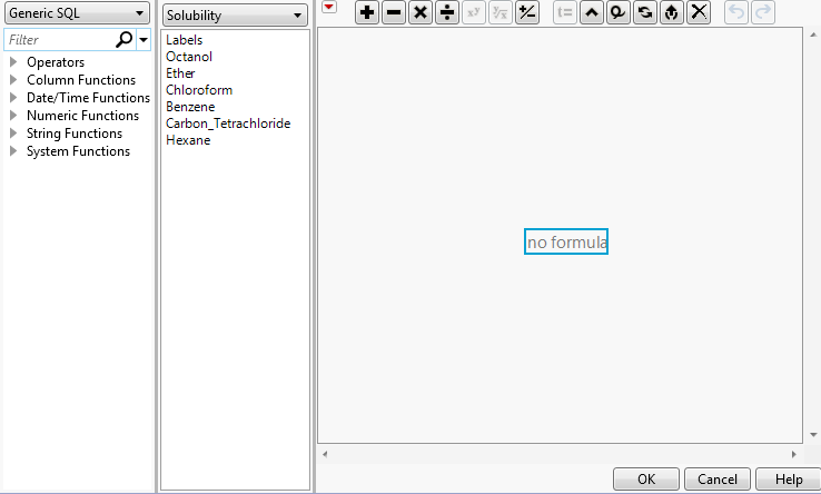
Use the WHERE Clause Editor
JMP provides help building WHERE clauses for SQL queries during ODBC import. It provides a WHERE clause editor that helps you build basic expressions using common SQL features, allowing vendor-specific functions. For example, you do not need to know whether SQL uses ‘=’ or ‘==’ for comparison, or avg() or average() for averaging.
In addition, string literals should be enclosed by single quotes (‘string’)rather than double quotes ("string").
To open the WHERE clause editor
1. Connect to a database by following the steps in Connect to a Database.
2. From the Database Open Table window, click the Advanced button.
3. Click the Where button.
USE the WHERE Clause Editor to add any of the following from the work panel: expressions, functions, and terms. They are applied to the highlighted blue box.
1. Click the Table Name Browser to select a table. The columns in that table appear in the list.
2. Click the SQL Vendor Name Browser to select the type of SQL that you want to use: GenericSQL, Access, DB2, MySQL, Oracle, SQL Server, or all of the above. Perform an action by clicking a function or operator in the list and selecting an operator from the list that appears.
Note: The following SQL Server data types are not supported: Binary, Geography, and Geometry.
3. Select an empty formula element in the formula editing area by clicking it. It is selected when there is a red outline around it. All terms within the smallest nesting box relative to the place that you clicked become selected. The subsequent actions apply to those combined elements.
4. Add operators to an expression by clicking buttons on the keypad.
5. (Optional) To customize your WHERE clause, select one of the options from the red triangle menu in the formula editor:
Show Boxing
Show or hide boxes around the WHERE clause terms.
Larger Font
Increase the font size of the formula.
Smaller Font
Decrease the font size of the formula.
Simplify
Simply the WHERE clause statement as much as possible.
Reset panel layout
Display the panels as shown in Figure 3.68.
The WHERE clause editor works similarly to the Formula Editor, which is described in Formula Editor.
Figure 3.68 The WHERE Clause Editor