Statistical Details for Bootstrapping
 Calculation of Fractional Weights
The Fractional Weights option is based on the Bayesian bootstrap (Rubin 1981). The number of times that an observation occurs in a given bootstrap sample is called its bootstrap weight. In the simple bootstrap, the bootstrap weights for each bootstrap sample are determined using simple random sampling with replacement.
In the Bayesian approach, sampling probabilities are treated as unknown parameters and their posterior distribution is obtained using a non-informative prior. Estimates of the probabilities are obtained by sampling from this posterior distribution. These estimates are used to construct the bootstrap weights, as follows:
• Randomly generate a vector of n values from a gamma distribution with shape parameter equal to (n - 1)/n and scale parameter equal to 1.
Note: Rubin (1981) uses 1 as the gamma shape parameter. The shape parameter that is used in JMP Pro ensures that the mean and variance of the fractional weights are equal to the mean and variance of the simple bootstrap weights.
• Compute S as the sum of the n values.
• Compute the fractional weights by multiplying the vector of n values by N / S, where N equals the number of rows or the sum of the frequencies if a Freq variable is specified.
Note: If a Freq variable is specified for the analysis, multiply the shape parameter for the gamma distribution by the Freq values on a row-by-row basis. The sum of the values of the Freq variable must be greater than 1. Then the shape parameters are equal to fi(N - 1)/N, where fi is the Freq value for the ith row and N equals the sum of the Freq values.
This procedure scales the fractional weights for each row to have mean and variance over bootstrap sampling equal to those of the simple bootstrap weights. The fractional bootstrap weights in each bootstrap sample are positive, sum to N, and have a mean of 1.
 Bias-Corrected Percentile Intervals
This section describes the calculation of the bias-corrected (BC) confidence intervals that appear in the Bootstrap Confidence Limits report when you run the Distribution script in the Bootstrap Results table. Bias-corrected percentile intervals improve on the ability of percentile intervals in accounting for asymmetry in the bootstrap distribution. See Efron (1981).
Notation
• p* is the proportion of bootstrap samples with an estimate of the statistic of interest that is less than or equal to the original estimate.
• z0 is the p* quantile of a standard normal distribution.
• zα is the α quantile of a standard normal distribution.
Bias-Corrected Confidence Interval Endpoints
The endpoints of a (1 - α) bias-corrected confidence intervals are given by quantiles of the bootstrap distribution:
• The lower endpoint is the following quantile:

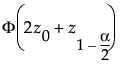
• The upper endpoint is the following quantile: