Supersaturated Screening Designs
It is common for brainstorming sessions to identify dozens of potentially active factors. Rather than reduce the list without the benefit of data, you can use a supersaturated design.
In a saturated design, the number of runs equals the number of model terms. In a supersaturated design, the number of model terms exceeds the number of runs (Lin, 1993). A supersaturated design can examine dozens of factors using fewer than half as many runs as factors. This makes it an attractive choice for factor screening when there are many factors and experimental runs are expensive.
Alternatively, use a group orthogonal supersaturated design for improved active effect identification over traditional supersaturated designs. See Group Orthogonal Supersaturated Designs.
Limitations of Supersaturated Designs
There are drawbacks to supersaturated designs:
• If the number of active factors is more than half the number of runs in the experiment, then it is likely that these factors will be impossible to identify. A general rule is that the number of runs should be at least four times larger than the number of active factors. In other words, if you expect that there might be as many as five active factors, you should plan on at least 20 runs.
• Analysis of supersaturated designs cannot yet be reduced to an automatic procedure. However, using forward stepwise regression is reasonable. In addition, the Screening platform (DOE >Classical > TwoLevel Screening > Fit Two Level Screening) offers a streamlined analysis.
Generate a Supersaturated Design
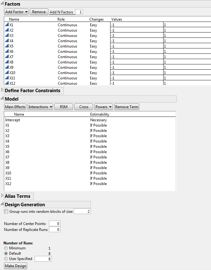
In this example, you want to construct a supersaturated design to study 12 factors in 8 runs. To create a supersaturated design, you set the Estimability of all model terms (except the intercept) to If Possible.
Note: This example is for illustration only. You should have at least 14 runs in any supersaturated design. If there are as many as four active factors, it is very difficult to interpret the results of an 8-run design. See Limitations of Supersaturated Designs.
1. Select DOE > Custom Design.
2. Type 12 next to Add N Factors.
3. Click Add Factor > Continuous.
4. Click Continue.
5. In the Model outline, select all terms except the Intercept.
6. Click Necessary next to any effect and change it to If Possible.
Setting the effects to If Possible ensures that JMP uses the Bayesian D-optimality criterion to obtain the design.
Figure 5.12 Factors, Model, and Number of Runs
7. In the Alias Terms outline, select all effects and click Remove Term.
This ensures that only the main effects appear in the Color Map on Correlations. This plot is constructed once the design is created.
8. Click the Custom Design red triangle and select Simulate Responses.
This option generates random responses that appear in your design table. You will use these responses to see how to analyze experimental data.
Keep the Number of Runs set to the Default of 8.
Note: Setting the Random Seed in step 9 and Number of Starts in step 10 reproduces the design shown in this example. In constructing a design on your own, these steps are not necessary.
9. (Optional) Click the Custom Design red triangle, select Set Random Seed, type 12345, and click OK.
10. (Optional) Click the Custom Design red triangle, select Number of Starts, type 5, and click OK.
11. Click Make Design.
12. Click Make Table.
Do not close your Custom Design window. You return to it later in this example.
Figure 5.13 Design Table with Simulated Responses
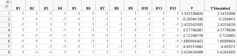
The response columns, Y and Y Simulated, are initiated with the same simulated values. The values are random values from a N(0, s) distribution. where s is the RMSE from the power analysis dialog with a default of 1. The Y Simulated values are updated with randomly generated values using the model defined by the parameter values in the Simulate Responses window. The Y column is intended for your true responses after the experiment has be run.
Figure 5.14 Simulate Responses Window
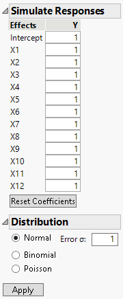
The Simulate Responses window shows default coefficients of 1 for all terms, a Normal distribution selection and Error σ of 1. The values in the Y and Y Simulated column currently reflect only random variation.
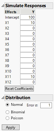
13. Change the values of the coefficients in the Simulate Responses window as shown in Figure 5.15.
Figure 5.15 Parameter Values for Simulated Responses
14. Click Apply.
The response values in the Y Simulated column change.
Note: The response values are randomly generated. Your values will not match those in Figure 5.16 exactly.
Figure 5.16 Y Simulated Response Column with X1 and X11 Active
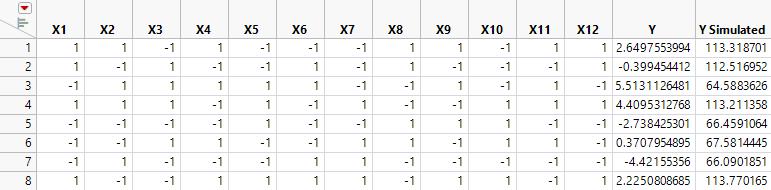
In your simulation, you specified X1 and X11 as active factors with large effects relative to the error variation. For this reason, your analysis of the data should identify these two factors as active.
Analyze a Supersaturated Design Using the Screening Platform
The Screening platform provides a way to identify active factors. Use the screening platform to analyze the Y Simulated values in the design table( Figure 5.16). The Screening platform is located under the DOE > Classical menu.
1. Select DOE > Classical > Two Level Screening > Fit Two Level Screening.
2. Select Y Simulated and click Y.
3. Select X1 through X12 ,click X and click OK.
Figure 5.17 Screening Report for Supersaturated Design
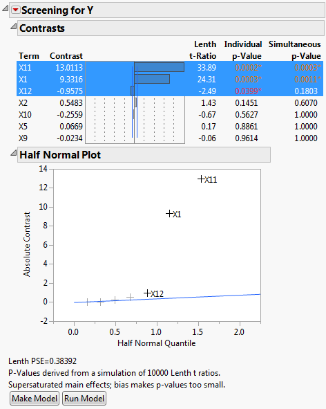
The factors X1 and X11 have large contrast and Lenth t-Ratio values. Also, their Simultaneous p-Values are small. In the Half Normal Plot, both X1 and X11 fall far from the line. The Contrasts and the Half Normal Plot reports indicate that X1 and X11 are active. Although X12 has an Individual p-Value less than 0.05, its effect is much smaller than that of X1 and X11.
Because the design is supersaturated, p-values might be smaller than they would be in a model where all effects are estimable. This is because effect estimates are biased by other potentially active main effects. In Figure 5.17, a note directly above the Make Model button warns you of this possibility.
You might also want to check whether the effects that appear active could be highly correlated with other effects. When this occurs, one effect can mask the true significance of another effect. The Color Map in Figure 5.19 displays absolute correlations between effects.
4. Click Make Model.
The constructed model contains only the effects X1, X11, and X12.
5. Click Run in the Model Specification window.
Figure 5.18 Parameter Estimates for Model
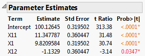
Note that the parameter estimates for X11 and X1 are close to the theoretical values that you used to simulate the model. See Figure 5.15, where you specified a model with X1 = 10 and X11 = 10. The significance of the factor X12 is an example of a false positive.
6. In your Custom Design window, open the Design Evaluation > Color Map on Correlations outline.
Figure 5.19 Color Map on Correlations Outline
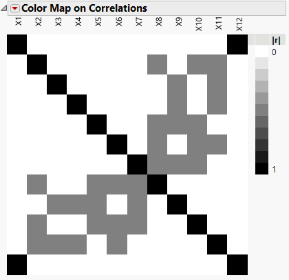
With your cursor, place your mouse pointer over cells to see the absolute correlations. Notice that X1 has correlations as high as 0.5 with other main effects (X4, X5, X7). (Figure 5.19 uses JMP default colors.)
Analyze a Supersaturated Design Using Stepwise Regression
Stepwise regression is another way to identify active factors. The design table in Figure 5.16 contains three scripts. The Model script analyzes your data using stepwise regression in the Fit Model platform.
1. In the Table panel of the design table, click the green triangle next to the Model script.
2. Change the Personality from Standard Least Squares to Stepwise.
3. Click Run.
4. In the Stepwise Fit for Y report, change the Stopping Rule to Minimum AICc.
For designed experiments, BIC is typically a more lenient stopping rule than AICc as it tends to allow inactive effects into the model.
5. Click Go.
Figure 5.20 Stepwise Regression for Supersaturated Design
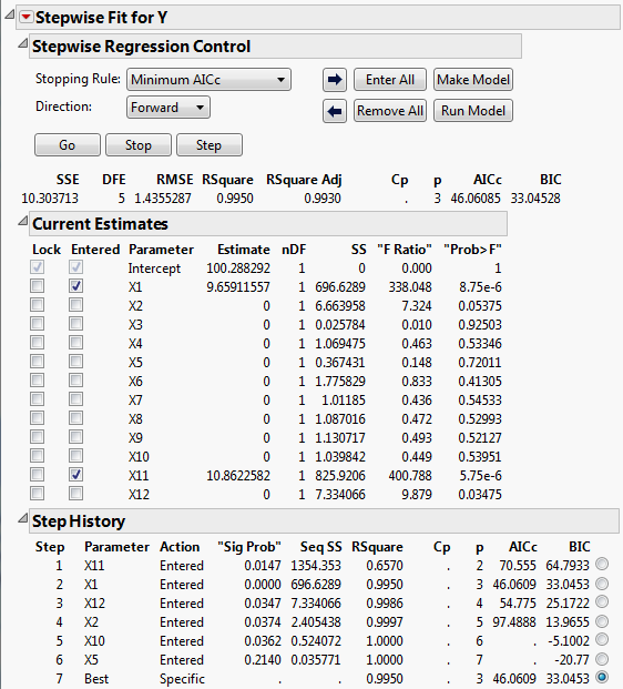
Figure 5.20 shows that the selected model consists of the two active factors, X1 and X11. The step history appears in the bottom part of the report. Keep in mind that correlations between X1 and X11 and other factors could mask the effects of other active factors (Figure 5.19).
Note: This example defines two large main effects and sets the rest to zero. Real-world situations can be less likely to have such clearly differentiated effects.