Transfer Function Models
Transfer Function
(Available only in the Transfer Function Analysis red triangle menu.) Shows the Transfer Function Model Specification window. Building a transfer function model is similar to building an ARIMA model; it is an iterative process of exploring, fitting, and comparing models. Before building a model and during the data exploration process, it is sometimes useful to prewhiten the data. See Prewhitening. For more information about transfer functions, see Statistical Details for Transfer Functions.
Note: Currently, the Transfer Function option has limited support of missing values. Because the Time Series platform also treats excluded rows as missing values, transfer function models cannot be fit on a data table with excluded rows.
Figure 17.7 Transfer Function Model Specification Window
![]()
The Transfer Function Model Specification window contains the following sections:
Noise Series Orders
Contains specifications for the noise series. Lowercase letters are coefficients for non-seasonal polynomials, and uppercase letters are coefficients for seasonal polynomials.
Choose Inputs
Enables you select the input series for the model.
Input Series Orders
Contains specifications for the input series. The first three orders relate to non-seasonal polynomials. The next four orders relate to seasonal polynomials. The final option is for an input lag.
There are three additional options that control model fitting:
Intercept
Specifies whether the model has an intercept. If unchecked, it is assumed that μ is zero.
Alternative Parameterization
Specifies whether the general regression coefficient is factored out of the numerator polynomials.
Constrain Fit
Toggles the constraining of the AR and MA coefficients.
Forecast Periods
Specifies the number of forecasting periods that are used for forecasting. If there are rows at the end of the data table that contain missing values for the Y variable and nonmissing values for the input variables, these rows are used in the initial forecasting settings. The values for the input variables are treated as future values of the input variables.
Prediction Interval
Specifies the confidence level for the prediction interval.
ARIMA Model Group
Shows the ARIMA Model Group window, which enables you to fit a range of ARIMA or Seasonal ARIMA models by specifying the range of orders. As you enter ranges into the window, the Total Number of Models updates accordingly.
Figure 17.8 ARIMA Model Group Specification Window
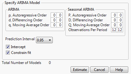
Once you specify the models and click Estimate, a Model Report for each specified model is added to the report window. See Reports.
Save Spectral Density
Creates a new data table containing the spectral density and periodogram where the (i+1)th row corresponds to the frequency fi = i / N (that is, the ith harmonic of 1 / N). The new data table has the following columns:
Period
The period of the ith harmonic, 1 / fi.
Frequency
The frequency of the harmonic, fi.
Angular Frequency
The angular frequency of the harmonic, 2πfi.
Sine
The Fourier sine coefficients, ai.
Cosine
The Fourier cosine coefficients, bi.
Periodogram
The periodogram, I(fi).
Spectral Density
The spectral density, a smoothed version of the periodogram.
Number of Forecast Periods
Shows a window that enables you to set the number of future periods that are forecast for the fitted models. The initial value is set in the Time Series launch window. All existing and future forecast results will use the new number of periods once it is changed.
Maximum Iterations
Shows a window that enables you to reset the maximum number of iterations for future optimizations used in fitting ARIMA models.
See Local Data Filter, Redo Menus, and Save Script Menus in Using JMP for more information about the following options:
Local Data Filter
Shows or hides the local data filter that enables you to filter the data used in a specific report.
Redo
Contains options that enable you to repeat or relaunch the analysis. In platforms that support the feature, the Automatic Recalc option immediately reflects the changes that you make to the data table in the corresponding report window.
Save Script
Contains options that enable you to save a script that reproduces the report to several destinations.
Save By-Group Script
Contains options that enable you to save a script that reproduces the platform report for all levels of a By variable to several destinations. Available only when a By variable is specified in the launch window.