Additional Example of the Time Series Platform
This example uses the SeriesP.jmp sample data table to show how to perform a time series analysis. You first create a new column that is appropriate for the Time ID.
Create Appropriate Time ID Column
1. Select Help > Sample Data Library and open Time Series/SeriesP.jmp.
The SeriesP.jmp data table contains a Year column and a Quarter column to identify the time period during which the responses were observed. However, the Time Series platform requires one column with unique, equally spaced time points to label the X axis. If no Time ID is specified, then the row number is used to identify the time periods. To avoid this and make the report easier to interpret, you construct a Time ID column from Year and Quarter.
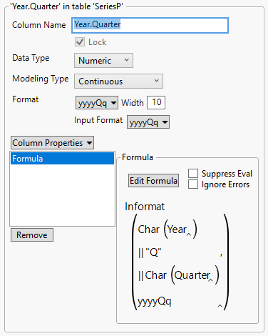
2. Select Cols > New Columns. In the Column Name box, type Year.Quarter.
3. Select Best > Date > yyyyQq next to Format.
4. Select Column Properties > Formula.
5. Click the gray triangle next to Date Time and click Informat.
6. Click the gray triangle next to Character.
7. Select Year, click Char, and then click Concat.
8. Type “Q” in the box (including quotation marks) and press the Enter key.
9. Click Concat.
10. Select Quarter and click Char.
11. Click the <formatName> box, type yyyyQq, and press the Enter key.
12. Click OK.
The completed New Column dialog box should appear as in Figure 17.16.
Figure 17.16 New Column
13. Click OK.
Note: This time column also works for X11 analyses.
Time Series Analysis
Now that the data table contains an appropriate Time ID column, proceed with the analysis.
1. Select Analyze > Specialized Modeling > Time Series.
2. Select GDP and click Y, Time Series.
3. Select Year.Quarter and click X, Time ID.
4. Click OK.
Figure 17.17 Time Series Report for SeriesP.jmp
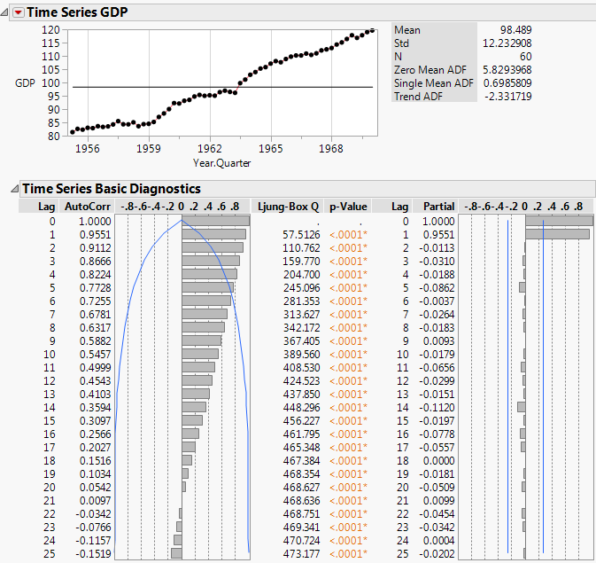
The series shows an increasing trend over time that is fairly linear. In addition, the autocorrelation chart shows that there is strong correlation between points that are close together. The AutoCorr values for points with lags of 1, 2, and 3 are 0.9551, 0.9112, 0.8666, respectively.
5. Click the Time Series GDP red triangle and select Difference.
6. Select 1 for the Nonseasonal Differencing Order and click Estimate.
Figure 17.18 Difference Report for SeriesP.jmp
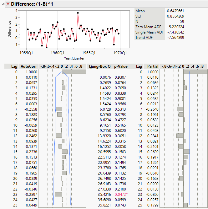
The Difference report helps determine an appropriate model to be fit to the original time series. The plot of differences shows that the differenced series no longer has the trend that was observed in the original data. This indicates that lag-1 differencing is an appropriate choice. Also, even after removing the trend, the series shows no sign of seasonality. For these reasons, models to fit the original series should be able to handle linear trends, but do not necessarily need to handle seasonality. Linear exponential smoothing and ARIMA models would be appropriate.
7. Click the Time Series GDP red triangle and select Smoothing Model > Linear Exponential Smoothing.
8. Click Estimate.
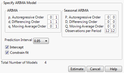
9. Click the Time Series GDP red triangle and select ARIMA Model Group. This enables you to fit multiple ARIMA models for a range of values of (p,d,q)(P,D,Q).
10. In the ARIMA box, set the following ranges:
– Fix d, the differencing order, at 1 by setting the range from 1 to 1 because the differencing report showed lag-1 differencing was appropriate.
– Set p, the autoregressive order, to range from 0 to 1 because the original series showed evidence of autocorrelation.
– Set q, the moving average order, to range from 0 to 1.
Note: In most cases, it is sufficient to keep p and q small.
– Leave P, D, and Q set at 0, since the series showed no evidence of seasonality.
These settings lead to the fitting of 4 total models.
Figure 17.19 ARIMA Model Group Specification
11. Click Estimate.
Figure 17.20 Model Comparison Table
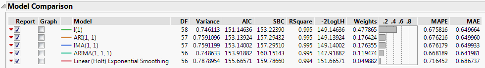
The Model Comparison Table is sorted such that the best fitting model, according to the AIC criterion, is at the top of the list. In this case, the ARIMA(0,1,0) model (denoted I(1) in the report) best fits the original time series. It should also be noted that although the I(1) model is “best,” all of the models have extremely similar values for the fit statistics. They could all be considered appropriate.
Figure 17.21 Model Report for ARIMA(0,1,0)
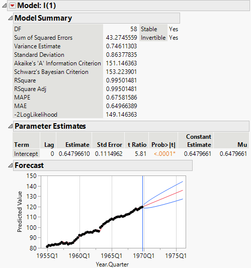
The model report for I(1) shows the forecast graph. The blue lines indicate the prediction intervals. GDP is predicted to continue increasing at a linear rate.