Comparisons
The Comparisons report section, shown in Figure 4.9, shows profilers for the selected distributions in the Nonparametric Overlay section, and includes the following tabs:
• Distribution
• Quantile
• Hazard
• Density
• Acceleration Factor
• Comparison Criterion
To show a specific profiler, select the appropriate distribution option in the Nonparametric Overlay section.
Profilers
The first five tabs show profilers for the selected distributions. Curves shown in the first four profilers correspond to both the time-to-event and explanatory variables. The Acceleration Factor profiler tab corresponds only to the acceleration factor (explanatory variable). Figure 4.9 shows the Distribution Profiler for the Weibull, Lognormal, Fréchet, and Loglogistic distributions.
Figure 4.9 Distribution Profiler
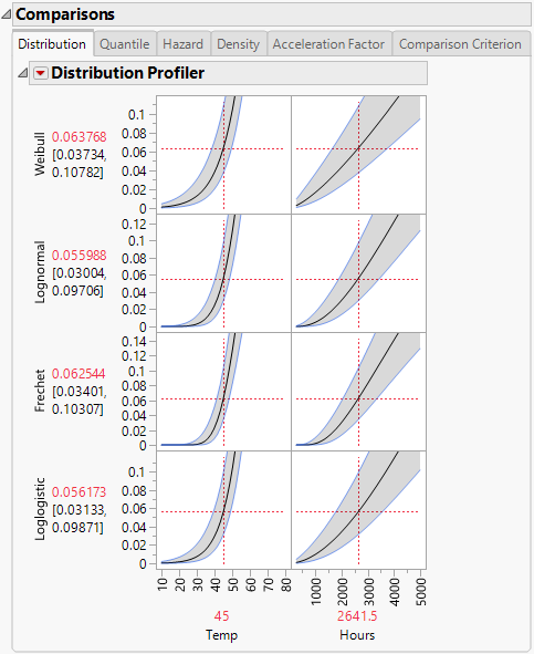
Comparable results appear on the Quantile, Hazard, and Density tabs. The Distribution, Quantile, Hazard, Density, and Acceleration Factor Profilers behave similarly to the Prediction Profiler in other platforms. For example, the vertical lines of Temp and Hours can be dragged to see how each of the distribution values change with temperature and time. For a detailed explanation of the Prediction Profiler, see Profiler in Profilers.
Quantile
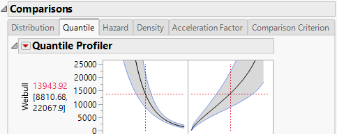
You can use the Quantile profiler for extrapolation. Suppose that the data are represented by a Weibull distribution. From viewing the Weibull Acceleration Factor Profiler in Figure 4.11, you see that the acceleration factor at 45 degrees Celsius is 17.18683 for a use condition temperature of 10 degrees Celsius. Select the Quantile tab to see the Quantile Profiler for the Weibull distribution. Select and drag the vertical line in the probability plot so that the probability reads 0.5. From viewing Figure 4.10, where the Probability is set to 0.5, you find that the quantile for the failure probability of 0.5 at 45 degrees Celsius is 13849.01 hours. So, at 10 degrees Celsius, you can expect that 50% of the units fail by 13849.01 * 17.18683 = 238021 hours.
Figure 4.10 Weibull Quantile Profiler for Devalt.jmp
Acceleration Factor
Selecting the Acceleration Factor tab shows the Acceleration Factor Profiler for the time-to-event variable for each specified distribution. To produce Figure 4.11, select Fit All Distributions from the Fit Life by X red triangle menu. Modify the use condition value for the explanatory variable by selecting Set Time Acceleration Use Condition from the Fit Life by X red triangle menu and entering the desired value. Note that the explanatory variable and the use condition value appear beside the profiler title.
Figure 4.11 Acceleration Factor Profiler for Devalt.jmp
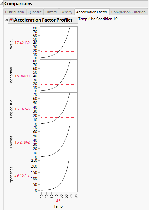
The Acceleration Factor Profiler lets you estimate time-to-failure for accelerated test conditions when compared with the use condition value and a parametric distribution assumption. The interpretation of a time-acceleration plot is generally the ratio of the pth quantile of the use condition to the pth quantile of the accelerated test condition. This relation applies only when the distribution is Lognormal, Weibull, Loglogistic, or Fréchet, and the scale parameter is constant for all levels. For more information about the parameterizations of the distributions, see Distributions in the Life Distribution section.
Note: The Acceleration Factor Profiler does not appear in the following instances: when the explanatory variable is discrete; the explanatory variable is treated as discrete; a customized formula does not use a unity scale factor; or the distribution is Normal, SEV, Logistic, or LEV.
Comparison Criterion
The Comparison Criterion tab shows the -2Loglikelihood, AICc, and BIC criteria for the distributions of interest. Figure 4.12 shows these values for the Weibull, Lognormal, Loglogistic, and Fréchet distributions. Distributions providing better fits to the data are shown at the top of the Comparisons report, sorted by AICc.
Figure 4.12 Comparison Criterion Report Tab
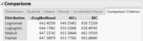
This report suggests that the Lognormal and Loglogistic distributions provide the best fits for the data, because the lowest criteria values are seen for these distributions. For a detailed explanation of the criteria, see Parametric Distributions in the Life Distribution section.