Competing Cause Details
For a competing cause model, a closed form for the aggregated distribution is given as follows:
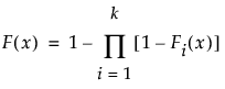
where the Fi(x), i = 1, …, k, are individual failure distributions corresponding to causes. Confidence limits are readily available, because all involved estimates are MLEs.
Specify a Fixed Parameter Model as a Distribution for a Cause
If a Fixed Parameter model is specified for a cause, you must fix the parameter in the Individual Causes report for that cause. Fix the parameter in the desired Parametric Estimate report in the Life Distribution - Failure Cause: <Name> report. The fixed parameter becomes part of the aggregated distribution when you click Update Model.
The following example illustrates how to include the Fixed Parameter model into the aggregated distribution:
1. Select Help > Sample Data Library and open Reliability/Appliance.jmp.
2. Select Analyze > Reliability and Survival > Life Distribution.
3. Select Time Cycles and click Y, Time to Event.
4. Select Cause Code and click Failure Cause.
5. Select Likelihood as the Confidence Interval Method.
6. Select Allow failure mode to use fixed parameter models.
7. Click OK.
Figure 3.25 Fixed Parameter Model with Cause 1 Omitted
By default, Cause = 1 is omitted, because there are not enough data. However, you do not want this cause to be omitted.
8. Open the Individual Causes report for Cause 1. The report is called Life Distribution - Failure Cause: 1 Failure Counts: 1.
9. Click the red triangle next to Parametric Estimate - Weibull and select Fix Parameter.
10. Select Weibull beta and type 2.
11. Click Update.
Figure 3.26 Fixed Parameter Model with Weibull Beta Specified
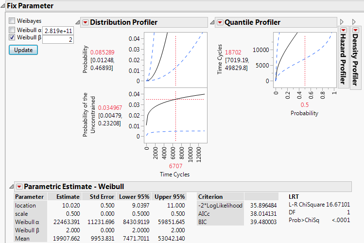
In the Parametric Estimate - Weibull report, assuming β equals 2, the alpha parameter is estimated to be 22463.391. Now you can use this for the failure distribution for Cause=1.
12. Scroll up to Cause Combination at the top of the report window.
13. Deselect Omit for Cause 1.
14. For the distribution for Cause 1, select Fixed Parameter Weibull.
15. Click Update Model.
Figure 3.27 Updated Model Showing Cause 1
Now the aggregated model uses the Fixed Parameter Weibull results for Cause 1 in the overall competing cause model.
Specify a Bayesian Model for a Cause
The steps for specifying a Bayesian model for a cause are similar to those described in Specify a Fixed Parameter Model as a Distribution for a Cause. Define the model in the desired Bayesian Estimation report found in the corresponding Parametric Estimate outline under Statistics in the Life Distribution report for the individual cause. See Bayesian Estimation - <Distribution Name>.
To incorporate a Bayesian model into the aggregated model, non-Bayesian distributions for other causes must be amenable to a simulation-based framework. For example, suppose that a model has two failure causes. One is modeled using a Weibull distribution and the other using a Bayesian approach for estimating the parameters of a second Weibull. The parameters for the first Weibull distribution, denoted by the vector θ1, are estimated using maximum likelihood. The parameters for the second Weibull, θ2, are estimated using the Bayesian approach.
The quantiles and median of the aggregated mixture distribution, denoted F(x, θ1, θ2), are obtained as follows:
• A parametric bootstrap is performed for the first Weibull, yielding random samples from the asymptotic distribution of the maximum likelihood estimate  . Denote a sampled value from the asymptotic distribution of
  by
by  .
.
• A sample is drawn from the posterior distribution of θ2, denoted by  .
.
• For each set of values  and
and  , an estimate of F(x, θ1, θ2), denoted by F*(x, θ1, θ2), is obtained.
• The values F*(x, θ1, θ2) are used to obtain estimates of the quantiles and median of the aggregated distribution. These are the values displayed in the Distribution profiler at a given value of x.
Specify a Weibayes Model for a Cause
The steps for specifying a Weibayes model for a cause are similar to those described in Specify a Fixed Parameter Model as a Distribution for a Cause. Select the Fix Parameter option in the Parametric Estimate - Weibull outline under Statistics in the Life Distribution report for the cause. In the Fix Parameter report, check the Weibayes option. The Weibayes model is treated as a Bayesian model and a bootstrap sample is drawn from the posterior distribution of the parameter alpha. See Liu and Wang (2013).
Mean Remaining Life Calculator
Use the Configuration option in the red triangle menu to set a value for the number of simulated failure times used in computing the mean remaining life. Denote this value by m.
To obtain an estimate of the mean remaining life at time t, m samples are drawn from the aggregated distribution conditioned on survival to time t. Their average is computed.
To compute the confidence limits for the mean remaining life, you must select the box in the Configuration window. You then have the option to set the number of bootstrap samples. Denote this value by n.
To compute the confidence interval, n samples of parameter estimates are drawn from either the asymptotic distributions of the MLEs, or the posterior distributions derived using Bayesian inference. For each sample of parameter values, an aggregated distribution is formed, from which m samples are drawn to compute a mean remaining life. The samples of n mean remaining life values are used to construct the confidence interval.
Fit Mixture Save Predictions Formulas
This section gives the formulas used in calculating values in the columns saved by the Fit Mixture report option Save Predictions.
Consider the following notation:
 is an estimate of the mixture proportion, wi
 is the estimated probability distribution function Fi
 is the estimated probability density function for Fi
• If the observation y is not censored, the saved value is given by the following:
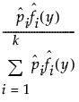
• If the observation is censored, the saved value is obtained by replacing the estimated density values in the formula for an uncensored observation by the following:
 for right censoring
 for left censoring
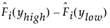 for interval censoring