 Construct Semiparametric Confidence Intervals for Variance Components
In this example, you are interested in the effects of temperature, time, and the amount of catalyst on a reaction. Temperature is a very-hard-to-change variable (whole plot factor), time is hard-to-change (subplot factor), and the amount of catalyst is easy-to-change. For information about whole plot and subplot factors, see Numbers of Whole Plots and Subplots in the Design of Experiments Guide.
Your goal is to obtain semiparametric confidence intervals for the whole-plot and sub-plot variance components. Previous studies have suggested that the whole-plot standard deviation is about twice the error standard deviation, and the sub-plot error is about 1.5 times the error standard deviation. The Wald intervals given in the REML report, which assume that the variance components are asymptotically normal, have poor coverage properties. You obtain confidence intervals using percentiles of the simulated distributions of the variance components.
This example contains the following tasks:
• Construct a custom design for your split-split-plot experiment. See Construct the Design.
• Fit a model using the REML method. See Fit the Model.
• Simulate variance component estimates in order to obtain percentile confidence intervals for the variance components. See Generate Confidence Intervals.
 Construct the Design
If you prefer to skip the steps in this section, select Help > Sample Data Library and open Design Experiment/Catalyst Design.jmp. In the Catalyst Design.jmp data table, click the green triangle next to the DOE Simulate script. Then go to Fit the Model.
1. Select DOE > Custom Design.
2. In the Factors outline, type 3 next to Add N Factors.
3. Click Add Factor > Continuous.
4. Double-click to rename these factors Temperature, Time, and Catalyst.
Keep the default Values of –1 and 1 for these factors.
5. For Temperature, click Easy and select Very Hard.
This defines Temperature to be a whole plot factor.
6. For Time, click Easy and select Hard for Time.
This defines Time to be a subplot factor.
7. Click Continue.
8. In the Model outline, select Interactions > 2nd.
This adds all two-way interactions to the model.
9. Click the Custom Design red triangle and select Simulate Responses.
This opens the Simulate Responses window after you select Make Table to construct the design table.
Note: Setting the Random Seed in step 10 and Number of Starts in step 11 reproduces the same design shown in this example. In constructing a design on your own, these steps are not necessary.
10. (Optional) Click the Custom Design red triangle and select Set Random Seed. Type 12345 and click OK.
11. (Optional) Click the Custom Design red triangle and select Number of Starts. Type 1000 and click OK.
12. Click Make Design.
13. Click Make Table.
Note: The entries in your Y and Y Simulated columns might differ from those that appear in Figure 10.2.
Figure 10.2 Design Table
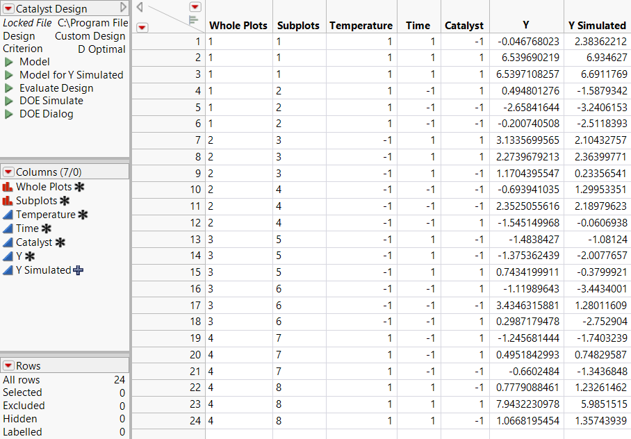
Figure 10.3 Simulate Responses Window
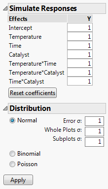
The design table and a Simulate Responses window appear. Notice that the design table contains a DOE Simulate script. At any time, you can run this script to specify different parameter values.
Continue to the next section, where you specify standard deviations for the whole plot and subplot errors, and fit a REML model to the first set of simulated values.
 Fit the Model
Assume that the whole plot and subplot errors are normal. Based on your estimates of their standard deviations, if the error standard deviation is about 1 unit, the whole plot standard deviation is about 2 units and the subplot standard deviation is about 1.5 units. Since you are interested only in the whole- and sub-plot variation, you do not need to change the values assigned to Effects in the Simulate Responses outline.
1. In the Distribution panel (Figure 10.3), next to Whole Plots σ, type 2.
Notice that the Normal distribution is selected by default. As a result, normal error is added to the formula.
2. Next to Subplots σ, type 1.5.
3. Click Apply.
In the data table, the formula for Y Simulated updates to reflect your specifications. To view the formula, click the plus sign to the right of the column name in the Columns panel.
4. In the data table, click the green triangle next to the Model script.
5. Click the Y variable next to the Y button and click Remove.
6. Click Y Simulated and click the Y button.
This action replaces Y with a column that contains a simulation formula.
7. Click Run.
The model that is fit is based on a single set of simulated responses.
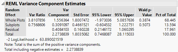
Note: Because the values in Y Simulated are randomly generated, the entries in your report might differ from those that appear in Figure 10.4.
Figure 10.4 REML Report Showing Wald Confidence Intervals
 Generate Confidence Intervals
Next, simulate values for the variance components and use these to construct simulated percentile confidence intervals.
1. In the REML Variance Components Estimates outline, right-click in the Var Component column and select Simulate.
Figure 10.5 Simulate Window
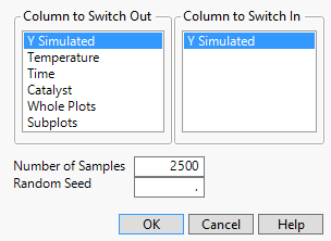
In your simulations, you replace the column Y Simulated, which you used to run your model, with a new instance of the column Y Simulated, which generates a new column of simulated values for each simulation. The column on which you right-clicked and that appears as selected, Var Component, is simulated for each effect listed in the Parameter Estimates table.
2. Next to Number of Samples, enter 200.
3. (Optional) Next to Random Seed, enter 456.
This reproduces the values shown in Figure 10.6, except for the values in row 1.
4. Click OK.
The entries in your row 1 might differ from those that appear in Figure 10.6.
Figure 10.6 Table of Simulated Results for Var Component (Partial View)
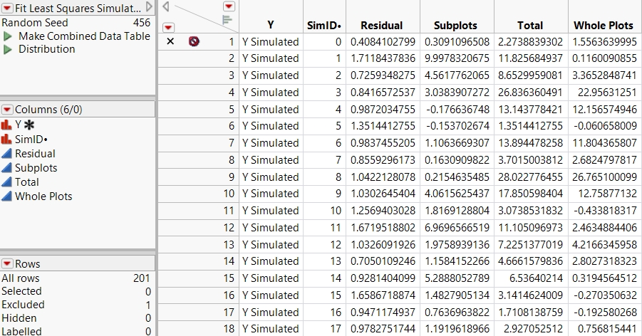
The first row of the Fit Least Squares Simulate Results (Var Component) data table contains the initial values of Var Component and is excluded. The remaining rows contain simulated values.
5. Run the Distribution script.
Figure 10.7 Distribution Plots for Variance Components (Partial View)
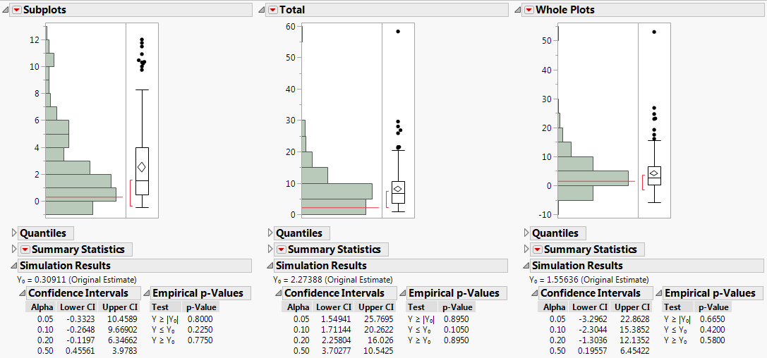
For each variance component, confidence intervals at various confidence levels are shown in the Simulation Results report. Compare the 95% intervals in the Alpha=0.05 row of each table to the intervals given in the REML report (Figure 10.4):
– The simulated 95% confidence interval for the whole-plot variance component is -3.296 to 22.863. The Wald interval given in the REML report is -1.973 to 5.086.
– The simulated 95% confidence interval for the sub-plot variance component is -0.332 to 10.459. The Wald interval given in the REML report is -0.605 to 1.223.
The intervals that you obtain using simulation are considerably wider than the REML interval calculated from your single set of values. For more precise intervals, consider running a larger number of simulations.