Extreme Vertices Design
An extreme vertices design requires restricted ranges on one or more of the factors, as defined by limits in the Factors panel or by linear constraints. An extreme vertices design consists of mixtures at the vertices of the factor space and at the averages of vertices up to a specified degree. The centroid point for two neighboring vertices joined by a line is a second-degree centroid. The centroid point for vertices sharing a plane is a third-degree centroid.
An Extreme Vertices Example with Range Constraints
To create an example extreme vertices design:
1. Select DOE > Classical > Mixture Design.
2. Under Factors, enter 2 for the number of additional factors to add and click Add.
3. Set the ranges for the five factors as shown in Figure 13.12 and click Continue.
Figure 13.12 Ranges for Five-factors
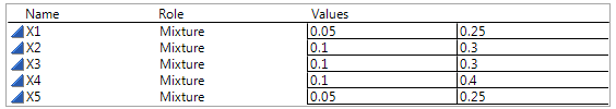
4. Enter 4 in the Degree text box and click Extreme Vertices.
Figure 13.13 Display and Modify Panel for Extreme Vertices Example
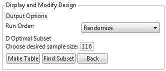
The default number of runs for this five-factor, degree 4 extreme vertices design is 116. This is the number of extreme vertices and averages up to degree 4 for these five factors given the constraints on their ranges. JMP uses the default set of mixtures as a candidate set to generate a smaller D Optimal design.
5. (Optional) To match the output of this example, click the Mixture Design red triangle and select Set Random Seed, and then enter 1409.
6. Enter 10 in the Choose desired sample size box and click Find Subset to generate the design.
Note: The Find Subset option uses the row exchange method (not coordinate exchange) to find the optimal subset of rows.
Figure 13.14 Ten Run D-optimal Extreme Vertices Design
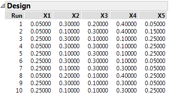
7. Click Make Table.
Visualize the Design
8. From the design table, select Graph >Ternary Plot.
9. Select X1, X2, X3, X4, and X5 and click X, Plotting, and then click OK.
Figure 13.15 Partial Output of Ternary Plot for Five-Factor Design
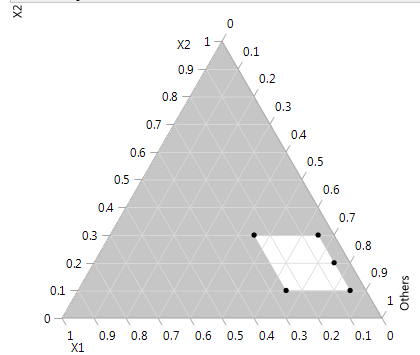
When you have more than three mixture components, the ternary plot shows a series of plots. Each plot has two component axes and the third axis is the sum of all other components. The plots are shaded if you have a constrained region. The unshaded portion represents the feasible region. For more information about ternary plots, see Ternary Plot Overview.
An Extreme Vertices Example with Linear Constraints
Consider the classic example presented by Snee (1979) and Piepel (1988). This example has three factors, X1, X2, and X3, with factor bounds and three linear constraints.
To create an extreme vertices design for this example:
1. Select DOE > Classical > Mixture Design.
2. Enter the values from Figure 13.16 for X1, X2, and X3 and click Continue.
Figure 13.16 Values and Linear Constraints for the Snee and Piepel Example
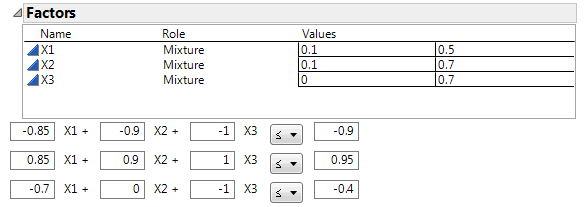
3. Click Linear Constraint three times. Enter the constraints as shown in Figure 13.16.
4. Click the Extreme Vertices button.
5. Click Make Table.
Visualize the Design
6. From the design table, select Graph >Ternary Plot.
7. Select X1, X2, and X3 and click X, Plotting, and then click OK.
Figure 13.17 Ternary Plot Showing Piepel Example with Constraints
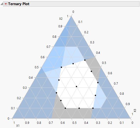
The ternary plot shows the feasible region as defined by the factor limits and the linear constraints. The design points are at the six vertices of the feasible region, at the six edge mid-points, and the overall centroid. For more information about ternary plots, see Ternary Plot Overview.
Statistical Details for Extreme Vertices Method
If there are linear constraints, JMP uses the CONSIM algorithm developed by R.E. Wheeler, described in Snee (1979) and presented by Piepel (1988) as CONVRT. The method is also described in Cornell (1990, Appendix 10a). The method combines constraints and checks to see whether vertices violate them. If so, it drops the vertices and calculates new ones. The method named CONAEV for doing centroid points is by Piepel (1988).
If there are no linear constraints (only range constraints), the extreme vertices design is constructed using the XVERT method developed by Snee and Marquardt (1974) and Snee (1975). After the vertices are found, a simplex centroid method generates combinations of vertices up to a specified order.
The XVERT method first creates a full 2nf – 1 design using the given low and high values of the nf – 1 factors with smallest range. Then, it computes the value of the one factor left out based on the restriction that the factors’ values must sum to one. It keeps points that are not in factor’s range. If not, it increments or decrements the value to bring it within range, and decrements or increments each of the other factors in turn by the same amount. This method keeps the points that still satisfy the initial restrictions.
The above algorithm creates the vertices of the feasible region in the simplex defined by the factor constraints. However, Snee (1975) has shown that it can also be useful to have the centroids of the edges and faces of the feasible region. A generalized n-dimensional face of the feasible region is defined by nf – n of the boundaries and the centroid of a face defined to be the average of the vertices lying on it. The algorithm generates all possible combinations of the boundary conditions and then averages over the vertices generated on the first step.