Optimality Criteria
This section provides information about the following designs:
D-Optimality
By default, the Custom Design platform optimizes the D-optimality criterion except when a full quadratic model is created using the RSM button. In that case, an I-optimal design is constructed.
The D-optimality criterion minimizes the determinant of the covariance matrix of the model coefficient estimates. It follows that D-optimality focuses on precise estimates of the effects. This criterion is desirable in the following cases:
• screening designs
• experiments that focus on estimating effects or testing for significance
• designs where identifying the active factors is the experimental goal
The D-optimality criterion is dependent on the assumed model. This is a limitation because often the form of the true model is not known in advance. The runs of a D-optimal design optimize the precision of the coefficients of the assumed model. In the extreme, a D-optimal design might be saturated, with the same number of runs as parameters and no degrees of freedom for lack of fit.
Specifically, a D-optimal design maximizes D, where D is defined as follows:
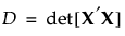
and where X is the model matrix as defined in Simulate Responses.
D-optimal split-plot designs maximize D, where D is defined as follows:
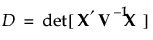
and V -1 is the block diagonal covariance matrix of the responses (Goos 2002).
Since a D-optimal design focuses on minimizing the standard errors of coefficients, it might not allow for checking that the model is correct. For example, a D-optimal design does not include center points for a first-order model. When there are potentially active terms that are not included in the assumed model, a better approach is to specify If Possible terms and to use a Bayesian D-optimal design.
Bayesian D-Optimality
Bayesian D-optimality is a modification of the D-optimality criterion. The Bayesian D-optimality criterion is useful when there are potentially active interactions or non-linear effects. See DuMouchel and Jones (1994) and Jones et al (2008).
Bayesian D-optimality estimates a specified set of model parameters precisely. These are the effects whose Estimability you designate as Necessary in the Model outline. But at the same time, Bayesian D-optimality has the ability to estimate other, typically higher-order effects, as allowed by the run size. These are the effects whose Estimability you designate as If Possible in the Model outline. To the extent possible given the run size restriction, a Bayesian D-optimal design allows for detecting inadequacy in a model that contains only the Necessary effects.
The Bayesian D-optimality criterion is most effective when the number of runs is larger than the number of Necessary terms, but smaller than the sum of the Necessary and If Possible terms. When this is the case, the number of runs is smaller than the number of parameters that you would like to estimate. Using prior information in the Bayesian setting allows for precise estimation of all of the Necessary terms while providing the ability to detect and estimate some If Possible terms.
To allow for a meaningful prior distribution to apply to the parameters of the model, responses and factors are scaled to have certain properties (DuMouchel and Jones, 1994, Section 2.2).
Consider the following notation:
• X is the model matrix as defined in Simulate Responses
• K is a diagonal matrix with values as follows:
– k = 0 for Necessary terms
– k = 1 for If Possible main effects, powers, and interactions involving a categorical factor with more than two levels
– k = 4 for all other If Possible terms
The prior distribution imposed on the vector of If Possible parameters is multivariate normal, with mean vector 0 and diagonal covariance matrix with diagonal entries 1/k2. Therefore, a value k2 is the reciprocal of the prior variance of the corresponding parameter.
The values for k are empirically determined. If Possible main effects, powers, and interactions with more than one degree of freedom have a prior variance of 1. Other If Possible terms have a prior variance of 1/16. In the notation of DuMouchel and Jones (1994) k = 1/τ.
To control the weights for If Possible terms, select Advanced Options > Prior Parameter Variance from the red triangle menu. See Advanced Options > Prior Parameter Variance.
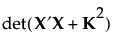
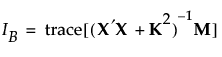
The posterior distribution for the parameters has the covariance matrix (X′X + K2)-1. The Bayesian D-optimal design is obtained by maximizing the determinant of the inverse of the posterior covariance matrix:
I-Optimality
I-optimal designs minimize the average variance of prediction over the design space. The I-optimality criterion is more appropriate than D-optimality if your primary experimental goal is not to estimate coefficients, but rather to do the following:
• predict a response
• determine optimum operating conditions
• determine regions in the design space where the response falls within an acceptable range
In these cases, precise prediction of the response takes precedence over precise estimation of the parameters.
The prediction variance relative to the unknown error variance at a point x0 in the design space can be calculated as follows:
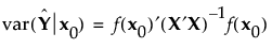
where X is the model matrix as defined in Simulate Responses.
I-optimal designs minimize the integral I of the prediction variance over the entire design space, where I is given as follows:
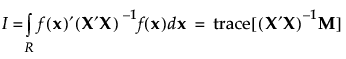
Here M is the moments matrix:
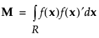
See Simulate Responses. For further information about simulating responses, see Goos and Jones (2011b).
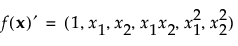
The moments matrix does not depend on the design and can be computed in advance. The row vector f (x)′ consists of a 1 followed by the effects corresponding to the assumed model. For example, for a full quadratic model in two continuous factors, f (x)′ is defined as follows:
A-Optimality
The A-optimality criterion minimizes the trace of the of the covariance matrix of the model coefficient estimates. The trace is the sum of the main diagonal elements of a matrix. An A-optimal design minimizes the sum of the variances of the regression coefficients.
Bayesian I-Optimality
The Bayesian I-optimal design minimizes the average prediction variance over the design region for Necessary and If Possible terms.
Consider the following notation:
• X is the model matrix, defined in Simulate Responses
• K is a diagonal matrix with values as follows:
– k = 0 for Necessary terms
– k = 1 for If Possible main effects, powers, and interactions involving a categorical factor with more than two levels
– k = 4 for all other If Possible terms
The prior distribution imposed on the vector of If Possible parameters is multivariate normal, with mean vector 0 and diagonal covariance matrix with diagonal entries 1/k2. (See Bayesian D-Optimality for more information about the values k.)
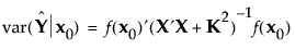
The posterior variance of the predicted value at a point x0 is as follows:
The Bayesian I-optimal design minimizes the average prediction variance over the design region, as follows:
where M is the moments matrix. See Simulate Responses.
Alias Optimality
Alias optimality seeks to minimize the aliasing between effects that are in the assumed model and effects that are not in the model but are potentially active. Effects that are not in the model but that are of potential interest are called alias effects. For more information about alias-optimal designs, see Jones and Nachtsheim (2011b).
Specifically, let X1 be the model matrix corresponding to the terms in the assumed model, as defined in Simulate Responses. The design defines the model that corresponds to the alias effects. Denote the matrix of model terms for the alias effects by X2.
The alias matrix is the matrix A, defined as follows:
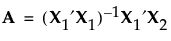
The entries in the alias matrix represent the degree of bias associated with the estimates of model terms. See The Alias Matrix in the Technical Details section for the derivation of the alias matrix.
The sum of squares of the entries in A provides a summary measure of bias. This sum of squares can be represented in terms of a trace as follows:

Designs that reduce the trace criterion generally have lower D-efficiency than the D-optimal design. Consequently, alias optimality seeks to minimize the trace of A′A subject to a lower bound on D-efficiency. For the definition of D-efficiency, see Optimality Criteria. The lower bound on D-efficiency is given by the D-efficiency weight, which you can specify under Advanced Options. See Advanced Options > D Efficiency Weight.