Power Analysis
Options relating to power calculations are available only for continuous-response models. These are the contexts in which power and related test details are available:
Parameter Estimate
To obtain retrospective test details for each parameter estimate, select Estimates > Parameter Power from the report’s red triangle menu. This option displays the least significant value, the least significant number, and the adjusted power for the 0.05 significance level test for each parameter based on current study data.
Effect or Effect Details
To obtain either prospective or retrospective details for the F test of a specific effect, select Power Analysis from the effect’s red triangle menu. Keep in mind that, for the Effect Screening and Minimal Report personalities, the report for each effect is found under Effect Details. For the Effect Leverage personality, the report for an effect is found to the right of the first (Whole Model) column in the report.
LS Means Contrast
To obtain either prospective or retrospective details for a test of one or more contrasts, select LSMeans Contrast from the effect’s red triangle menu. Define the contrasts of interest and click Done. From the Contrast red triangle menu, select Power Analysis.
Custom Test
To obtain either prospective or retrospective details for a custom test, select Estimates > Custom Test from the response’s red triangle menu. Define the contrasts of interest and click Done. From the Custom Test red triangle menu, select Power Analysis.
In all cases except the first, selecting Power Analysis opens the Power Details window. You then enter information in the Power Details window to modify the calculations according to your needs.
Effect Size
The effect size, denoted by δ, is a measure of the difference between the null hypothesis and the true values of the parameters involved. The null hypothesis might be formulated in terms of a single linear contrast that is set equal to zero, or of several such contrasts. The value of δ reflects the difference between the true values of the contrasts and their hypothesized values of 0.
In general terms, the effect size is given by:
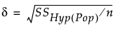
where  is the sum of squares for the hypothesis being tested given in terms of population parameters and n is the total number of observations.
When observations are available, the estimated effect size is calculated by substituting the calculated sum of squares for the hypothesis into the formula for δ.
Balanced One-Way Layout
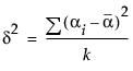
For example, in the special case of a balanced one-way layout with k levels where the ith group has mean response αi,
Recall that JMP codes parameters so that, for i =1, 2,..., k-1

and
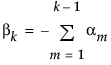
So, in terms of these parameters, δ for a two-level balanced layout is given by:
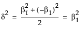
or 
Unbalanced One-Way Layout
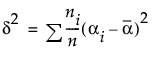
In the case of an unbalanced one-way layout with k levels, and where the ith group has mean response αi and ni observations, and where  :
:
Effect Size and Power
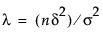
The power is the probability that the F test of a hypothesis is significant at the α significance level, when the true effect size is a specified value. If the true effect size equals δ, then the test statistic has a noncentral F distribution with noncentrality parameter
When the null hypothesis is true (that is, when the effect size is zero), the noncentrality parameter is zero and the test statistic has a central F distribution.
The power of the test increases with λ. In particular, the power increases with sample size n and effect size δ, and decreases with error variance σ2.
Some books, such as Cohen (1977), use a standardized effect size, Δ = δ/σ, rather than the raw effect size used by JMP. For the standardized effect size, the noncentrality parameter equals λ = nΔ2.
In the Power Details window, δ is initially set to  . SSHyp is the sum of squares for the hypothesis, and n is the number of observations in the current study. SSHyp is an estimate of δ computed from the data, but such estimates are biased (Wright and O’Brien 1988). To calculate power using a sample estimate for δ, you might want to use the Adjusted Power and Confidence Interval calculation rather than the Solve for Power calculation. The adjusted power calculation uses an estimate of δ that is partially corrected for bias. See Computations for the Adjusted Power in the Statistical Details section.
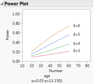
Plot of Power by Sample Size
To see a plot of power by sample size, select the Power Plot option from the red triangle menu at the bottom of the Power report. JMP plots the Power and Number columns from the Power table. The plot shown in Figure 3.69 results from plotting the Power table obtained in Example of Retrospective Power Analysis.
Figure 3.69 Plot of Power by Sample Size
The Least Significant Number (LSN)
The least significant number (LSN) is the smallest number of observations that leads to a significant test result, given the specified values of delta, sigma, and alpha. Recall that delta, sigma, and alpha represent, respectively, the effect size, the error standard deviation, and the significance level.
Note: LSN is not a recommendation of how large a sample to take because it does not take into account the probability of significance. It is computed based on specified values of delta and sigma.
The LSN has these characteristics:
• If the LSN is less than the actual sample size n, then the effect is significant.
• If the LSN is greater than n, the effect is not significant. If you believe that more data will show essentially the same structural results as does the current sample, the LSN suggests how much data you would need to achieve significance.
• If the LSN is equal to n, then the p-value is equal to the significance level alpha. The test is on the border of significance.
• The power of the test for the effect size, calculated when n = LSN, is always greater than or equal to 0.5. Note, however, that the power can be close to 0.5, which is considered low for planning purposes.
The Least Significant Value (LSV)
The LSV, or least significant value, is computed for single-degree-of-freedom hypothesis tests. These include tests for the significance of individual model parameters, as well as more general linear contrasts. The LSV is the smallest effect size, in absolute value, that would be significant at level alpha. The LSV gives a measure of the sensitivity of the test on the scale of the parameter, rather than on a probability scale.
The LSV has these characteristics:
• If the absolute value of the parameter estimate or contrast is greater than or equal to the LSV, then the p-value of the significance test is less than or equal to alpha.
• The absolute value of the parameter estimate or contrast is equal to the LSV if and only if its significance test has p-value equal to alpha.
• The LSV is the radius of a 1 – α confidence interval for the parameter or linear combination of parameters. The 1 – α confidence interval is centered at the estimate of the parameter or contrast.
Power
The power of a test is the probability that the test gives a significant result. The power is a function of the effect size δ, the significance level α, the error standard deviation σ, and the sample size n. The power is the probability that you will detect a specified effect size at a given significance level. In general, you would like to design studies that have high power of detecting differences that are of practical or scientific importance.
Power has these characteristics:
• If the true value of the parameter is in fact the hypothesized value, the power equals the significance level of the test. The significance level is usually a small value, such as 0.05. The small value is appropriate, because you want a low probability of seeing a significant result when the postulated hypothesis is true.
• If the true value of the parameter is not the hypothesized value, in general, you want the power to be as large as possible.
• Power increases as: sample size increases; error variance decreases; the difference between the true parameter value and the hypothesized value increases.
The Adjusted Power and Confidence Intervals
In retrospective power analysis, you typically substitute sample estimates for the population parameters involved in power calculations. This substitution causes the noncentrality parameter estimate to have a positive bias (Wright and O’Brien 1988). The adjusted power calculation is based on a form of the estimated noncentrality parameter that is partially corrected for this bias.
You can also construct a confidence interval for the adjusted power. Such confidence intervals tend to be wide. See Wright and O’Brien (1988).
Note that the adjusted power and confidence interval calculations are relevant only for the value of δ estimated from the data (the value provided by default). For other values of delta, the adjusted power and confidence interval are not provided.
See Computations for the Adjusted Power in the Statistical Details section.
Example of Retrospective Power Analysis
This example illustrates a retrospective power analysis using the Big Class.jmp sample data table. The Power Details window (Figure 3.70) permits exploration of various quantities over ranges of values for α, σ, δ, and Number, or study size. Clicking Done replaces the window with the results of the calculations.
1. Select Help > Sample Data Library and open Big Class.jmp.
2. Select Analyze > Fit Model.
3. Select weight and click Y.
4. Add age, sex, and height as the effects.
5. Click Run.
6. Click the age red triangle and select Power Analysis.
Figure 3.70 Power Details Window for Age
7. Replace the δ value in the From box with 3, and enter 6 and 1 in the To and By boxes as shown in Figure 3.70.
8. Replace the Number value in the From box with 20, and enter 60 and 10 in the To and By boxes as shown in Figure 3.70.
9. Select Solve for Power and Solve for Least Significant Number.
10. Click Done.
11. The Power Details window is replaced by the Power Details report.
Figure 3.71 Power Details Report for Age
This analysis is a retrospective power analysis because the calculations assume a study with a structure identical to that of the Big Class.jmp sample data table. For example, the calculation of power in this example depends on the effects entered into the model and the number of participants in each age and sex grouping. Also, the value of σ was derived from the current study, though you could have replaced it with a value that would be representative of a future study.
For more information about the power results shown in Figure 3.71, see Power. For more information about the least significant number (LSN), see The Least Significant Number (LSN).
Prospective Power Analysis
Prospective analysis helps you answer the question, “If differences of a specified size exist, will I detect them given my proposed sample size, alpha level, and estimate of error variance?” In a prospective power analysis, you must provide estimates of the group means and sample sizes in a data table. You must also provide an estimate of the error standard deviation σ in the Power Details window.
Equal Group Sizes
Consider a situation where you are comparing the means of three independent groups. To obtain sample sizes to achieve a given power, select DOE > Sample Size and Power and then select k Sample Means. Next to Std Dev, enter your estimate of the error standard deviation. In the Prospective Means list, enter means that reflect the smallest differences that you want to detect. If, for example, you want to detect a difference of 8 units between any two means, enter the extreme values of the means (for example, 40, 40, and 48). Because the power is based on deviations from the grand mean, you can enter only values that reflect the desired differences (for example, 0, 0, and 8).
If you click Continue, you obtain a graph of power versus sample size. If instead you specify either power or sample size in the Sample Size window, the other quantity is computed and displayed in the Sample Size window. In particular, if you specify power, the sample size that is provided is the total required sample size. The k Sample Means calculation assumes equal group sizes. For three groups, you would divide the sample size by 3 to obtain the individual group sizes. For more information about k Sample Means, see k Sample Means Calculator in the Design of Experiments Guide.
Unequal Group Sizes
Suppose that you want to design a study that uses groups of different sizes. You need to plan an experiment to study two treatments that reportedly reduce bacterial counts. You want to compare the effect of these treatments with results from a control group that receives no treatment. You also want to detect a difference of at least 8 units between the means of either treatment group and the control group. But the control group must be twice as large as either treatment group. The two treatment groups also must be equal in size. Previous studies suggest that the error standard deviation is on the order of 5 or 6.
To obtain a prospective power analysis for this situation, create a data table containing some basic information, as shown in the Bacteria.jmp sample data table.
Figure 3.72 Bacteria.jmp Data Table
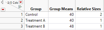
• The Group column identifies the groups.
• The Means column reflects the smallest difference among the columns that it is important to detect. Here, it is assumed that the control group has a mean of about 40. You want the test to be significant if either treatment group has a mean that is at least 8 units higher than the mean of the control group. For this reason, you assign a mean of 48 to one of the two treatment groups. Set the mean of the other treatment group equal to that of the control group. (Alternatively, you could assign the control group and one of the treatment groups means of 0 and the remaining treatment group a mean of 8.) Note that the differences in the group means are population values.
• The Relative Sizes column shows the desired relative sizes of the treatment groups. This column indicates that the control group needs to be twice as large as each of the treatment groups. (Alternatively, you could start out with an initial guess for the treatment sizes that respects the relative size criterion.)
Note: The Relative Sizes column must be assigned the role of a Freq (frequency). See the symbol to the right of the column name in the Columns panel.
Next, use Fit Model to fit a one-way analysis of variance model (Figure 3.73). Note that Relative Sizes is declared as Freq in the launch window. Also, the Minimal Report emphasis option is selected.
Figure 3.73 Fit Model Launch Window for Bacteria Study
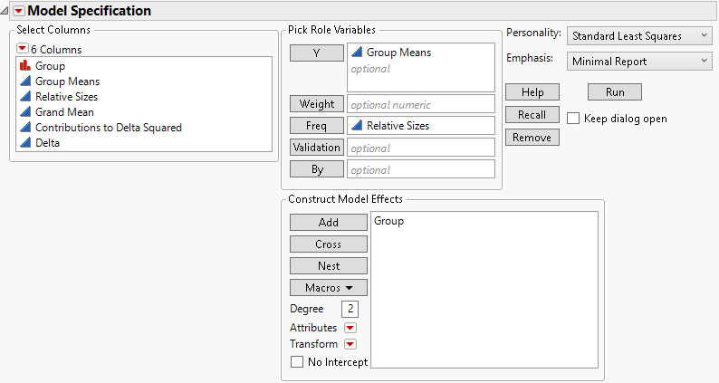
Click Run to obtain the Fit Least Squares report. The report shows Root Mean Square Error and Sum of Squares for Error as 0.0, because you specified a data table with no error variation within the groups. You must enter a proposed range of values for the error variation to obtain the power analysis. Specifically, you have information that the error variation will be about 5 but might be as large as 6.
1. Click the disclosure icon next to Effect Details to open this report.
2. Click the Group red triangle and select Power Analysis.
3. To explore the range of error variation suspected by the scientist, under σ, enter 5 in the first box and 6 in the second box (Figure 3.74).
4. Note that δ is entered as 3.464102. This is the effect size that corresponds to the specified difference in the group means. The data table contains three hidden columns that illustrate the calculation of the effect size. (See Unbalanced One-Way Layout.)
5. To explore power over a range of study sizes, under Number, enter 16 in the first box, 64 in the second box, and an increment of 4 in the third box (Figure 3.74).
6. Select Solve for Power.
7. Click Done.
Figure 3.74 Power Details Window for Bacteria Study
The Power Details report, shown in Figure 3.75, replaces the Power Details window. This report gives power calculations for α = 0.05, for all combinations of σ = 5 and 6, and sample sizes of 16 to 64 in increments of size 4. When σ is 5, to obtain about 90% power, you need a total sample size of about 32. You need 16 participants in the control group and 8 in each of the treatment groups. On the other hand, if σ is 6, then a total of 44 participants is required.
Figure 3.75 Power Details Report for Bacteria Study
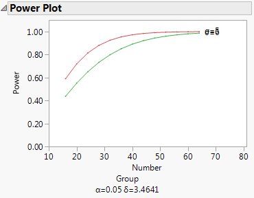
Click the arrow at the bottom of the table in the Power Details report to obtain a plot of power versus sample size for the two values of σ, shown in Figure 3.76. Here, the red markers correspond to σ = 5 and the green correspond to σ = 6.
Figure 3.76 Power Plot for Bacteria Study