Split Plot Design Example
Levels of random effects are randomly selected from a larger population of levels. For the purpose of inference, the distribution of a random effect is assumed to be normal, with mean zero and some variance (called a variance component).
In a sense, every model has at least one random effect, which is the effect that makes up the residual error. The individual observations are assumed to be randomly selected from a much larger population, and the error term is assumed to have a mean of zero and variance σ2.
The most common random effects model is the repeated measures or split plot model. Table 4.2 lists the types of effects in a split plot model. In these models, the experiment has two layers. Some effects are applied on the whole plots or subjects of the experiment. Then these plots are divided or the subjects are measured at different times and other effects are applied within those subunits. The effects describing the whole plots or subjects are whole plot effects, and the subplots or repeated measures are subplot effects. Usually, the subunit effect is omitted from the model and absorbed as residual error.
|
Split Plot Model |
Type of Effect |
Repeated Measures Model |
|---|---|---|
|
whole plot treatment |
fixed effect |
across subjects treatment |
|
whole plot ID |
random effect |
subject ID |
|
subplot treatment |
fixed effect |
within subject treatment |
|
subplot ID |
random effect |
repeated measures ID |
Each of these cases can be treated as a layered model, and there are several traditional ways to fit them in a fair way. The situation is treated as two different experiments:
1. The whole plot experiment has whole plot or subjects as the experimental unit to form its error term.
2. Subplot treatment has individual measurements for the experimental units to form its error term (left as residual error).
The older, traditional way to test whole plots is to do any one of the following:
• Take means across the measurements and fit these means to the whole plot effects.
• Form an F-ratio by dividing the whole plot mean squares by the whole plot ID mean squares.
• Organize the data so that the split or repeated measures form different columns. Fit a MANOVA model, and use the univariate statistics.
These approaches work if the structure is simple and the data are complete and balanced. However, there is a more general model that works for any structure of random effects. This more generalized model is called the mixed model, because it has both fixed and random effects.
The most common type of layered design is a balanced split plot, often in the form of repeated measures across time. One experimental unit for some of the effects is subdivided (sometimes by time period) and other effects are applied to these subunits.
Consider the data in the Animals.jmp sample data table (the data are fictional). The study collected information about differences in the seasonal hunting habits of foxes and coyotes. Each season for one year, three foxes and three coyotes were marked and observed periodically. The average number of miles that they wandered from their dens during different seasons of the year was recorded (rounded to the nearest mile). The model is defined by the following aspects:
• The continuous response variable called miles
• The species effect with values fox or coyote
• The season effect with values fall, winter, spring, and summer
• An animal identification code called subject, with nominal values 1, 2, and 3 for both foxes and coyotes
There are two layers to the model:
1. The top layer is the between-subject layer, in which the effect of being a fox or coyote (species effect) is tested with respect to the variation from subject to subject.
2. The bottom layer is the within-subject layer, in which the repeated-measures factor for the four seasons (season effect) is tested with respect to the variation from season to season within a subject. The within-subject variability is reflected in the residual error.
The season effect can use the residual error for the denominator of its F statistics. However, the between-subject variability is not measured by residual error and must be captured with the subject within species (subject[species]) effect in the model. The F statistic for the between-subject effect species uses this nested effect instead of residual error for its F ratio denominator.
Note: JMP Pro users can construct this model using the Mixed Model personality.
To specify the split plot model for this data, follow these steps:
1. Select Help > Sample Data Library and open Animals.jmp.
2. Select Analyze > Fit Model.
3. Select miles and click Y.
4. Select species and subject and click Add.
5. In the Select Columns list, select species.
6. In the Construct Model Effects list, select subject.
7. Click Nest.
This adds the subject within species (subject[species]) effect to the model.
8. Select the nested effect subject[species].
9. Select Attributes > Random Effect.
This nested effect is now identified as an error term for the species effect and appears as subject[species]&Random.
10. In the Select Columns list, select season and click Add.
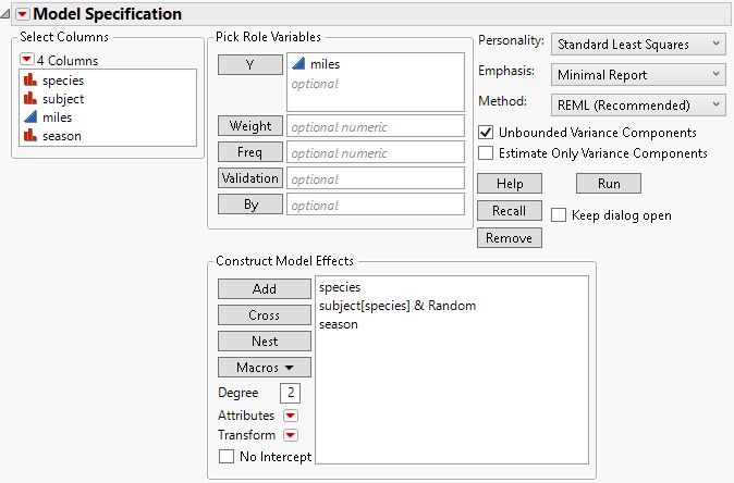
When you define an effect as random using the Attributes menu, the Method options (REML and EMS) appear at the top right of the dialog. The REML option is selected as the default. The completed launch window is shown in Figure 4.19.
Figure 4.19 Fit Model Dialog
11. Click Run.
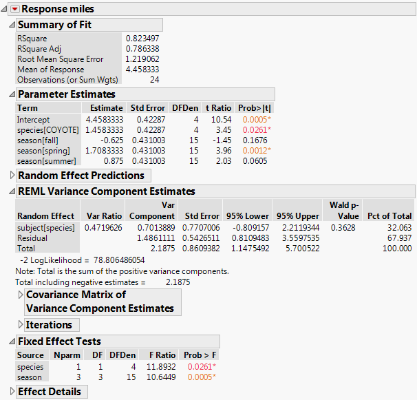
The report is shown in Figure 4.20. Both fixed effects, species and season, are significant. The REML Variance Component Estimates report gives estimates of the subject within species and residual variances.
Figure 4.20 Partial Report of REML Analysis