The Missing Value Report
Figure 20.13 Missing Value Report for Continuous Variables in Arrhythmia.jmp.
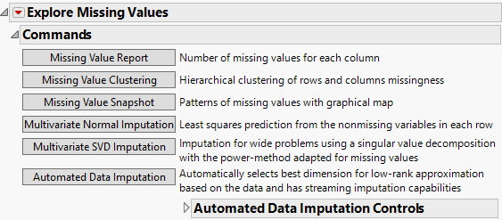
After you click OK in the launch window, the report opens to show a Commands outline and a Missing Columns report. The commands are the following:
• Multivariate Normal Imputation (Not available if you entered a Numeric column with a Nominal or Ordinal modeling type in the launch window.)
• Multivariate SVD Imputation (Not available if you entered a Numeric column with a Nominal or Ordinal modeling type in the launch window.)
•  Automated Data Imputation (Not available if you entered a Numeric column with a Nominal or Ordinal modeling type in the launch window.)
Tip: To run a missing value command across all levels of a By variable, hold down the Ctrl key and click the desired command button.
Missing Value Report
The Missing Value Report opens the Missing Columns report, which lists the name of each column and the number of missing values in that column.
Show only columns with missing
Removes columns from the list that do not have missing values.
Close
Closes the Missing Columns report.
Select Rows
Selects the rows in the data table that contain missing values for the column(s) that you select in the Missing Columns report.
Exclude Rows
Applies the excluded row state for rows in the data table that contain missing values for the column(s) that you select in the Missing Columns report.
Color Cells
Colors the cells in the data table that contain missing values for the column(s) that you select in the Missing Columns report.
Color Rows
Colors the rows in the data table that contain missing values for the column(s) that you select in the Missing Columns report.
Missing Value Clustering
Missing Value Clustering provides a hierarchical clustering analysis of the missing data.
• The dendrogram to the right of the plot shows clusters of missing data pattern rows. These are the rows that you would obtain by using Tables > Missing Data Pattern.
• The dendrogram beneath the plot shows clusters of variables.
Use this report to determine whether certain groups of columns tend to have similar patterns of missing values.
The rows of the plot are defined by the missing data patterns; there is a row for each pattern. The columns correspond to the variables. Each red cell indicates a group of missing values for the column listed beneath the plot. Place your cursor in a cell to see the list of values represented. Click in the plot to select missing data pattern rows. Vertical bars are displayed to indicate the selected patterns.
Missing Value Snapshot
The Missing Value Snapshot shows a cell plot for the missing values. The columns represent the variables. Black cells indicate a missing value. This plot is especially useful in understanding missingness for longitudinal data, where subjects can withdraw from a study before the end of the data collection period.
Multivariate Normal Imputation
The Multivariate Normal Imputation utility imputes missing values based on the multivariate normal distribution. The procedure requires that all variables have a Continuous modeling type. The algorithm uses least squares imputation. The covariance matrix is constructed using pairwise covariances. The diagonal entries (variances) are computed using all nonmissing values for each variable. The off-diagonal entries for any two variables are computed using all observations that are nonmissing for both variables. In cases where the covariance matrix is singular, the algorithm uses minimum norm least squares imputation based on the Moore-Penrose pseudo-inverse.
Multivariate Normal Imputation allows the option to use a shrinkage estimator for the covariances. The use of shrinkage estimators is a way of improving the estimation of the covariance matrix. For more information about shrinkage estimators, see Schäfer and Strimmer (2005).
Note: If a validation column is specified, the covariance matrices are computed using observations from the Training set.
Multivariate Normal Imputation Report
The imputation report explains the results of the multivariate imputation process. Results include the following:
• Method of imputation (either least squares or minimum-norm least squares)
• How many values were replaced
• Shrinkage estimator on/off
• Factor by which the off-diagonals were scaled
• How many rows and columns were affected
• How many different missing value patterns there were
Once the imputation is complete, the cells corresponding to imputed values in the data table are colored in light blue. If the Missing Columns report is open, it is updated to show no missing values.
Click Undo to undo the imputation and replace the imputed data with missing values.
Multivariate SVD Imputation
The Multivariate SVD Imputation utility imputes missing values using the singular value decomposition (SVD). This utility is useful for data with hundreds or thousands of variables. Because SVD calculations do not require calculation of a covariance matrix, the SVD method is recommended for wide problems that contain large numbers of variables. The procedure requires that all variables have a Continuous modeling type.
The singular value decomposition represents a matrix of observations X as X = UDV′, where U and V are orthogonal matrices and D is a diagonal matrix.
The SVD algorithm used by default in the Multivariate SVD Imputation utility is the sparse Lanczos method, also known as the implicitly restarted Lanczos bidiagonalization method (IRLBA). See Baglama and Reichel (2005). The algorithm does the following:
1. Each missing value is replaced with its column’s mean.
2. An SVD decomposition is performed on the matrix of observations, X.
3. Each cell that had a missing value is replaced by the corresponding element of the UDV′ matrix obtained from the SVD decomposition.
4. Steps 2 and 3 are repeated until the SVD converges to the matrix X.
Imputation Method Window
When you click Multivariate SVD Imputation, the Imputation Method window shows the recommended settings.
Number of Singular Vectors
Number of singular vectors that are computed and used in the imputation.
Note: It is important not to specify too many singular vectors, otherwise the SVD and the imputations do not change from iteration to iteration.
Maximum Iterations
The number of iterations used in imputing the missing values.
Show Iteration Log
Opens a Details report that shows the number of iterations and gives details about the criteria.
For large problems, a progress bar shows how many dimensions the SVD has completed. You can stop the imputation and use that number of dimensions at any time.
Multivariate SVD Imputation Report
The imputation report explains the results of the multiple imputation process.
• Method of imputation
• How many values were replaced
• How many rows and columns were affected
Once the imputation is complete, the Missing Columns report is automatically shown indicating no missing values in the columns that were imputed. Imputed values are displayed in light blue.
Click Undo to undo the imputation and replace the imputed data with missing values.
 Automated Data Imputation
The Automated Data Imputation (ADI) utility imputes missing values using a low-rank matrix approximation method, also known as matrix completion. Once trained, the ADI model is capable of performing missing data imputations for streaming data through scoring formulas. Streaming data are added rows of observations that become available over time and were not used for tuning or validating the imputed model. This utility is flexible, robust, and automated to select the best dimension for the low-rank approximation. These features enable ADI to work well for many different types of data sets. The procedure requires that all variables have a Continuous modeling type.
A low-rank approximation of a matrix is of the form X = UDV′ and can be viewed as an extension of singular value decomposition (SVD). ADI uses the Soft-Impute method as the imputation model and is designed such that the data determines the rank of the low-rank approximation.
The ADI algorithm performs the following steps:
1. The data are partitioned into training and validation sets.
2. Each set is centered and scaled using the observed values from the training set.
3. For each partitioned data set, additional missing values are added within each column and are referred to as induced missing (IM) values.
4. The imputation model is fit on the training data set along a solution path of tuning parameters. The IM values are used to determine the best value for the tuning parameter.
5. Additional rank reduction is performed using the training data set by de-biasing the results from the chosen imputation model in step 4.
6. Final rank reduction is performed to calibrate the model for streaming data and to prevent overfitting. This is done by fitting the imputation model on the validation set, using the rank determined in step 5 as an upper bound.
Automated Data Imputation Controls
The ADI utility contains options for saving the imputed values and advanced controls.
Figure 20.14 ADI Controls
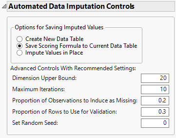
Options for Saving Imputed Values
The following three options for saving the imputed values for the ADI method are available:
Create New Data Table
Creates a new data table that has the same dimensions as the original data table. In the new data table, the columns selected in the launch window contain the imputed values.
Save Scoring Formula to Current Data Table
Saves a column group, named Imputed_, to the current data table that contains the imputed columns specified in the launch window. A hidden column, ADI Impute Column, is also added to the current data table that contains the imputed vectors and the scoring formula used in the data imputation. The column formulas automatically update if any additional rows are added to the data table, enabling missing data imputation for streaming data. This is the default option.
Impute Values in Place
Imputes the missing values in the current data table. The imputed values are displayed in light blue.
Advanced Controls
Contains the following advanced controls, which default to recommended settings based on the data:
Dimension Upper Bound
Determines the maximum rank allowed in the low-rank approximation. This is determined by the dimension of the matrix formed by the chosen columns.
Maximum Iterations
Determines the number of values that are iterated over to determine the tuning parameter for the imputation model. The default is 10.
Proportion of Observations to Induce as Missing
Determines the proportion of IM values that are added to the training and validation sets. The default proportion for each set is 0.2.
Proportion of Rows to Use for Validation
Determines the proportion of rows to use in the training and validation sets. The default proportion for the validation set is 0.3.
Set Random Seed
Determines the random seed for ADI. Use this option to obtain reproducible results.