Analysis of Covariance with Unequal Slopes Example
Continuing with the Drug.jmp sample data table, this example fits a model where the slope for the covariate depends on the level of Drug. After fitting the model, the example compares the least square means for the levels of Drug at a specific value of the covariate x.
1. Select Help > Sample Data Library and open Drug.jmp.
2. Select Analyze > Fit Model.
3. Select y and click Y.
4. Select both Drug and x and click Macros > Factorial to Degree.
This adds terms up to the degree specified in the Degree box to the model. The default value for Degree is 2. Thus, the main effects of Drug and x, and their interaction, Drug*x, are added to the model effects list.
5. Click Run.
This specification adds two columns to the linear model (call them x4i and x5i) that allow the slopes for the covariate to differ by Drug level. The new variables are formed by multiplying the indicator variables for Drug by the covariate values, giving the following formula:

Table 4.1, shows the coding for this model. The mean of X is 10.7333. It is used in centering continuous terms.
Regressor | Effect | Values |
X1 | Drug[a] | +1 if a, 0 if d, –1 if f |
X2 | Drug[d] | 0 if a, +1 if d, –1 if f |
X3 | X | the values of X |
X4 | Drug[a]*(X - 10.733) | X – 10.7333 if a, 0 if d, –(X – 10.7333) if f |
X5 | Drug[d]*(X - 10.733) | 0 if a, X – 10.7333 if d, –(X – 10.7333) if f |
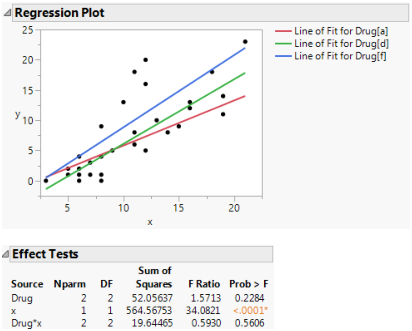
A portion of the report is shown in Figure 4.6. The Regression Plot shows fitted lines with different slopes. The Effect Tests report gives a p-value for the interaction of 0.56. This is not significant, indicating the model does not need to include different slopes.
Figure 4.6 Plot with Interaction
Perform a Spotlight Analysis
You now want to compare the least square means for the levels of Drug at a specific value of the covariate x. This type of comparison in an analysis of covariance model is sometimes referred to as spotlight analysis. For more information about spotlight analysis, see Spiller et al. (2013).
1. Click the Response y red triangle and select Estimates > Multiple Comparisons.
2. In the Multiple Comparisons window, select User-Defined Estimates.
3. Select all three values below Choose Drug Levels.
4. In the first box below x, enter 12.5.
5. Click Add Estimates.
This adds comparisons of the three levels of Drug at x = 12.5.
6. Click OK.
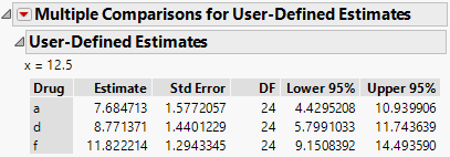
The User-Defined Estimates report shows least square means estimates for each level of Drug with the covariate x set to 12.5. The red triangle next to Multiple Comparisons for User-Defined Estimates contains options that enable you to test for differences among the estimates.
Figure 4.7 User-Defined Estimates Report
7. Click the red triangle next to Multiple Comparisons for User-Defined Estimates and select Comparisons with Overall Average.
Figure 4.8 Comparisons with Overall Average Decision Chart
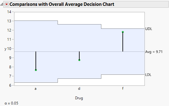
The Comparisons with Overall Average option creates an analysis of means (ANOM) chart for differences between the average and the three least squares means. From the ANOM chart, you conclude that there is not a significant effect of Drug on the response at x = 12.5.