Bézier Curves
A complete discussion of Bézier curves is beyond the scope of the Scripting Guide. JSL has several commands for defining and drawing curves and their associated meshes.
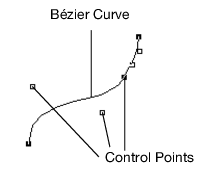
Figure 13.19 Bézier Curve
One-Dimensional Evaluators
To define a one-dimensional map, use the Map1 command.
Map1( target, u1, u2, stride, order, matrix )
The target argument defines what the control points represent. Values of the target argument are shown in Table 13.6. Note that you must use the Enable command to enable the argument.
target Argument | Meaning |
|---|---|
MAP1_VERTEX_3 | (x, y, z) vertex coordinates |
MAP1_VERTEX_4 | (x, y, z, w) vertex coordinates |
MAP1_INDEX | color index |
MAP1_COLOR_4 | R, G, B, A |
MAP1_NORMAL | normal coordinates |
MAP1_TEXTURE_COORD_1 | s texture coordinates |
MAP1_TEXTURE_COORD_2 | s, t texture coordinates |
MAP1_TEXTURE_COORD_3 | s, t, r texture coordinates |
MAP1_TEXTURE_COORD_4 | s, t, r, q texture coordinates |
The second two arguments (u1 and u2) define the range for the map. The stride value is the number of values in each block of storage. In other words, the value is the offset between the beginning of one control point and the beginning of the next control point. The order should equal the degree of the curve plus one. The matrix holds the control points.
For example, Map1( MAP1_VERTEX_3, 0, 1, 3, 4, <4x3 matrix> ) is typical for setting the two end points and two control points to define a Bézier line.
You use the MapGrid1 and EvalMesh1 commands to define and apply an evenly spaced mesh.
MapGrid1( un, u1, u2 )
sets up the mesh with un divisions spanning the range u1 to u2. Code is simplified by using the range 0 to 1.
EvalMesh1( mode, i1, i2 )
actually generates the mesh from i1 to i2. The mode can be either POINT or LINE. The EvalMesh1 command makes its own Begin and End clause.
The following example script demonstrates a one-dimensional outlier. A random set of control points draws a smooth curve. Only the first and last points are on the curve. Using NPOINTS=4 results in a cubic Bézier spline.
boxwide = 500;boxhigh = 400;gridsize = 100; // bigger for finer divisions
/* We suggest you use only values between 2 and 8 (inclusively). Numbers beyond these might be interpreted differently, depending on implementation. This value is the degree+1 of the fitted curve */
NPOINTS = 4;point = J( NPOINTS, 3, 0 );
// create an array of x,y,z triples
For( x = 1, x <= NPOINTS, x++,
point[x, 1] = (x - 1) / (NPOINTS - 1) - .5;
// x from -.5 to +.5
point[x, 2] = Random Uniform() - .5; // y is random in same range
// z is always zero, which causes the curve to stay in a plane
point[x, 3] = 0;
);
spline = Scene Box( boxwide, boxhigh );// data from -.5 to .5 in x and y; this is a little larger
spline << Ortho( -.6, .6, -.6, .6, -2, 2 );
spline << Enable( MAP1_VERTEX_3 );spline << MapGrid1( gridsize, 0, 1 );
spline << Color( .2, .2, 1 ); // blue curve
spline << Map1( MAP1_VERTEX_3, 0, 1, 3, NPOINTS, point );
spline << Line Width( 2 ); // not-so-skinny curve
spline << EvalMesh1( LINE, 0, gridsize ); // also try LINE, POINT
spline << Color( .2, 1, .2 );
spline << Point Size( 4 ); // big fat green points
// show the points and label them
For( i = 1, i <= NPOINTS, i++,
spline << Begin( "POINTS" );
spline << Vertex( point[i, 1], point[i, 2], point[i, 3] );
spline << End; spline << Push Matrix;spline << Translate( point[i, 1], point[i, 2], point[i, 3] );
spline << Text( center, bottom, .05, Char( i ) );
spline << Pop Matrix;);
New Window( "Spline", spline );
https://www.tinaja.com/glib/bezconn.pdf offers an explanation of connecting cubic segments so that both the slope and the rate of change match at the connection point. This example does not illustrate doing so; there is only one segment here.