Binomial Generalized Regression Example
This example shows how to develop a prediction model for the binomial response, Severity, in the Liver Cancer.jmp sample data table.
1. Select Help > Sample Data Library and open Liver Cancer.jmp.
2. Select Analyze > Fit Model.
3. Select Severity from the Select Columns list and click Y.
4. Select BMI through Jaundice and click Macros > Factorial to Degree.
All terms up to degree 2 (the default in the Degree box) are added to the model.
5. From the Personality list, select Generalized Regression.
The Distribution list automatically shows the Binomial distribution. This is the only distribution available when Y is binary and has a Nominal modeling type.
6. Click Run.
The Generalized Regression report that appears contains a Model Comparison report, a Model Launch control panel, and a Logistic Regression report. Note that the default estimation method is the Lasso.
7. Select Elastic Net as the Estimation Method.
8. Select the Adaptive box.
9. Click Go.
A Binomial Adaptive Elastic Net with AICc Validation report appears. The Solution Path is shown in Figure 7.3.
Figure 7.3 Solution Path Plot
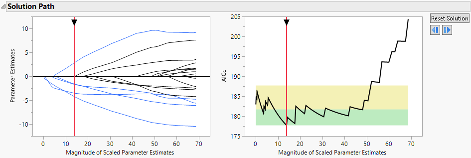
The paths for terms that have nonzero coefficients are shown in blue. The optimal parameter values are substantially shrunken away from the MLE. The Validation Plot to the right indicates that several models can be considered as good as the best model. To view those models, slide the vertical red bar around in the region where the black line is in the green area.
10. Click the red triangle next to Binomial Adaptive Elastic Net with AICc Validation and select the Select Zeroed Terms option.
The 16 terms that have coefficient estimates of zero are highlighted in the Parameter Estimates for Original Predictors report. The Effect Tests report designates these terms as Removed.
The Effect Tests report also shows that there are no significant terms at the 0.05 level. However, the Time*Markers interaction has a small p-value of 0.0626 and the Time effect has a small p-value of 0.1458.
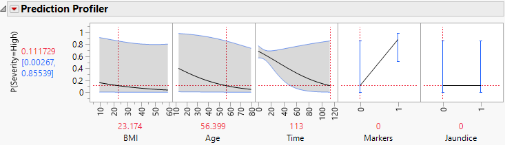
11. Click the red triangle next to Binomial Adaptive Elastic Net with AICc Validation and select Profilers > Profiler.
Figure 7.4 Profiler for Probability That Severity = High, Time Low
Examine the Prediction Profiler to see how Time and the Time*Markers interaction affect Severity.
Note: The predictor Hepatitis is not shown in the profiler because it does not appear in any active (nonzero) terms. Because Markers and Jaundice appear in active interaction terms, they appear in the profiler even though, as main effects, they are not active.
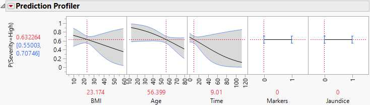
12. Move the red dashed line for Time from left to right to see its interaction with Markers (Figure 7.4 and Figure 7.5). For patients who enter the study with small values of Time since diagnosis, Markers have little impact on Severity. But for patients who enter the study having been diagnosed for a longer time, Markers are important. For those patients, normal markers suggest a lower probability of high Severity.
Figure 7.5 Profiler for Probability That Severity = High, Time High