 Correlated Response Example
In this example, the effect of two layouts dealing with wafer production is studied for a characteristic of interest. Each of 50 wafers is partitioned into four quadrants and the characteristic is measured on each of these quadrants. Data of this type are usually presented in a format where each row contains all of the repeated measurements for one of the units of interest. Data of this type are often analyzed using separate models for each response. However, when repeated measurements are taken on a single unit, it is likely that there is within-unit correlation. Failure to account for this correlation can result in poor decisions and predictions. You can use the Mixed Model personality to account for and model the possible correlation.
For Mixed Model analysis of repeated measures data, each repeated measurement needs to be in its own row. If your data are in the typical format where all repeated measurements are in the same row, you can construct an appropriate data table for Mixed Model analysis by using Tables > Stack. See Stack Columns in the Using JMP.
In this example, you first fit univariate models using the usual data table format. Then you use the Mixed Model personality to fit models for the four responses while simultaneously accounting for possible correlation among the responses.
 Fit Univariate Models
Use Standard Least Squares to fit a univariate model for each of the four quadrants.
1. Select Help > Sample Data Library and open Wafer Quadrants.jmp.
This data table is structured for Mixed Model analysis, with one row for each Y measurement on each Quadrant. To conduct univariate analyses, you split the table using a saved script.
2. In the Wafer Quadrants.jmp data table, click the green triangle next to the Split Y by Quadrant script.
The new data table is in the format often used to record repeated measures data. Each value of Wafer ID defines a row and the four measurements for that wafer are given in the single row.
3. Select Analyze > Fit Model.
Since there is a Model script in the data table, the Model Specification window is already filled in. Note that the columns High, High through Low, Low are entered as Y and that Layout is the single model effect.
4. Click Run.
Figure 8.38 Four Univariate Models
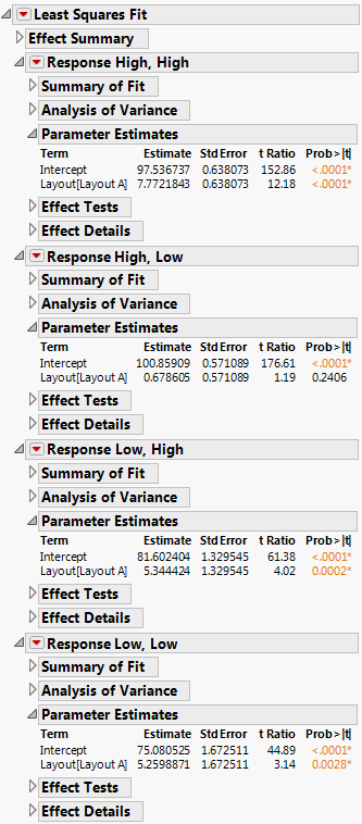
The report indicates that Layout has a statistically significant effect for all quadrants except the High, Low quadrant.
 Perform Mixed Model Analysis
Using the Mixed Model analysis, you can obtain more information.
1. Return to Wafer Quadrants.jmp. Or, if you have closed it, select Help > Sample Data Library and open Wafer Quadrants.jmp.
2. Select Analyze > Fit Model.
3. Select Y and click Y.
4. Select Mixed Model from the Personality list.
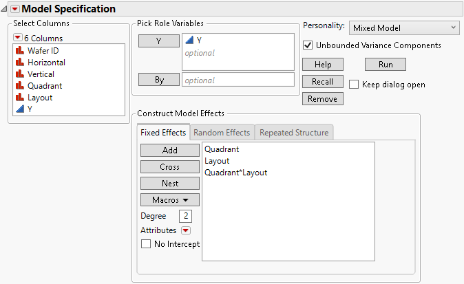
5. Select Quadrant and Layout from the Select Columns list and click Macros > Full Factorial.
This model specification enables you to explore the effect of Layout on the repeated measurements as well as the possible interaction of Layout with Quadrant.
Figure 8.39 Fit Model Launch Window Showing Completed Fixed Effects Tab
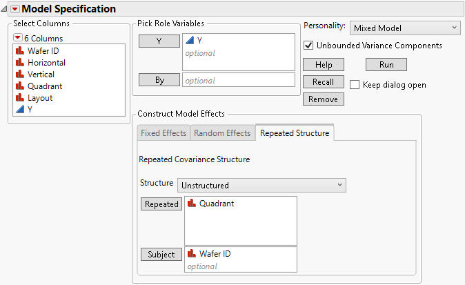
6. Select the Repeated Structure tab.
7. Select Unstructured from the Structure list.
8. Select Quadrant and click Repeated.
9. Select Wafer ID and click Subject.
Figure 8.40 Fit Model Launch Window Showing Repeated Structure Tab
10. Click Run.
Figure 8.41 Fit Mixed Report with Fixed Effects Parameter Estimates Report Closed
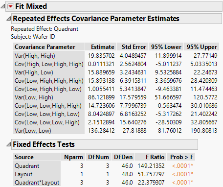
The Repeated Effects Covariance Parameter Estimates report gives the estimated variances and covariances for the four responses. Note that the confidence interval for the covariance of Low, High with High, High does not include zero. This suggests that there is a positive covariance between measurements in these two quadrants. This is information that the Mixed Model analysis uses and that is not available when the responses are modeled independently.
The Fixed Effects Tests report indicates that there is a significant Layout by Characteristic interaction.
 Explore the Layout by Characteristic Interaction with the Profiler
1. Click the Fit Mixed red triangle and select Marginal Model Inference > Profiler.
2. In the Profiler plot, compare the predicted values for Y across the quadrants by first setting the vertical red dotted line at Layout A and then at Layout B.
Figure 8.42 Profile for Quadrant for Layout A
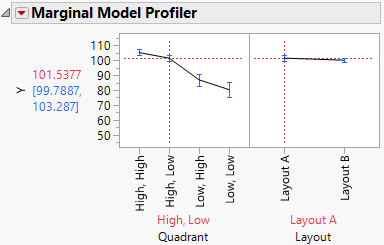
Figure 8.43 Profile for Quadrant for Layout B
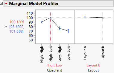
The differences in the profiles at each setting of Layout give you insight into the significant interaction. It appears that the interaction is partially driven by the differences for the High, High quadrant.
 Plot of Y by Layout and by Quadrant
Use Graph Builder to explore the nature of the interaction.
1. Click the Fit Mixed red triangle and select Save Columns > Prediction Formula.
The prediction formula is saved to the data table in the column Pred Formula Y.
2. Select Graph > Graph Builder.
3. Drag Horizontal to the X zone.
4. Drag Vertical to the Y zone.
5. Drag Pred Formula Y to the Color zone.
6. Drag Layout to the Wrap zone.
7. Click Done to hide the control panel.
Figure 8.44 Completed Graph Builder Plot
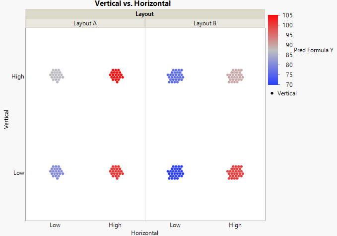
Note: Because the points in Graph Builder are randomly jittered, your plot might not match Figure 8.44 exactly.
The plot shows the predicted differences for the eight Layout and Quadrant combinations using a color intensity scale. The predicted values for the High, Low quadrant are in the lower right. The color gradient shows relatively little difference for these predicted values. Other differences are clearly indicated.