Distributions
This section provides details for the distributional fits in the Life Distribution platform. Meeker and Escobar (1998, ch. 2-5) is an excellent source of theory, application, and discussion for both the nonparametric and parametric details that follow.
Estimation and Confidence Intervals
The parameters of all distributions, unless otherwise noted, are estimated using maximum likelihood estimates (MLEs). The only exceptions are the threshold distributions. If the smallest observation is an exact failure, then this observation is treated as interval-censored with a small interval. The parameter estimates are the MLEs estimated from this slightly modified data set. Without this modification, the likelihood can be unbounded, so an MLE might not exist. This approach is similar to that described in Meeker and Escobar (1998, p. 275), except that only the smallest exact failure is censored. This is the minimal change to the data that guarantees boundedness of the likelihood function.
The Life Distribution platform offers two methods for calculating confidence intervals for the distribution parameters. These methods are labeled as Wald or Likelihood and can be selected in the launch window for the Life Distribution platform. Wald confidence intervals are used as the default setting. The computations for the confidence intervals for the cumulative distribution function (cdf) start with Wald confidence intervals on the standardized variable. Next, the intervals are transformed to the cdf scale (Nelson 1982, pp. 332–333 and pp. 346-347). The confidence intervals given in the other graphs and profilers are transformed Wald intervals (Meeker and Escobar 1998, ch. 7). Joint confidence intervals for the parameters of a two-parameter distribution are shown in the log-likelihood contour plots. They are based on approximate likelihood ratios for the parameters (Meeker and Escobar 1998, ch. 8).
Nonparametric Fit
A nonparametric fit describes the basic curve of a distribution. For data with no censoring (failures only) and for data where the observations consist of both failures and right-censoring, JMP uses Kaplan-Meier estimates. For mixed, interval, or left censoring, JMP uses Turnbull estimates. When your data set contains only right-censored data, the Nonparametric Estimate report indicates that the nonparametric estimate cannot be calculated.
The Life Distribution platform uses the midpoint estimates of the step function to construct probability plots. The midpoint estimate is halfway between (or the average of) the current and previous Kaplan-Meier estimates.
Parametric Distributions
Parametric distributions provide a more concise distribution fit than nonparametric distributions. The estimates of failure-time distributions are also smoother. Parametric models are also useful for extrapolation (in time) to the lower or upper tails of a distribution.
Note: Many distributions in the Life Distribution platform are parameterized by location and scale. For lognormal fits, the median is also provided. A threshold parameter is also included in threshold distributions. Location corresponds to μ, scale corresponds to σ, and threshold corresponds to γ.
Lognormal
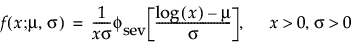
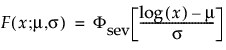
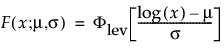
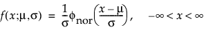
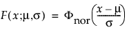
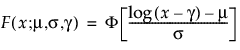
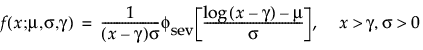
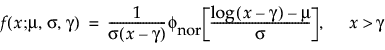
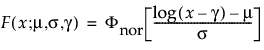
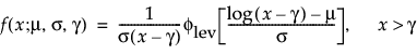
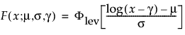
Lognormal distributions are used commonly for failure times when the range of the data is several powers of 10. This distribution is often considered as the multiplicative product of many small positive identically independently distributed random variables. It is reasonable when the log of the data values appears normally distributed. Examples of data appropriately modeled by the lognormal distribution include hospital cost data, metal fatigue crack growth, and the survival time of bacteria subjected to disinfectants. The pdf curve is usually characterized by strong right-skewness. The lognormal pdf and cdf are:
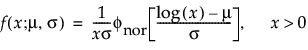

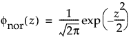
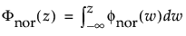
where
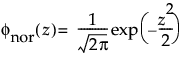
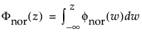
and

are the pdf and cdf, respectively, for the standardized normal, or nor(μ = 0, σ = 1) distribution.
Weibull
The Weibull distribution can be used to model failure time data with either an increasing or a decreasing hazard rate. It is used frequently in reliability analysis because of its tremendous flexibility in modeling many different types of data, based on the values of the shape parameter, β. This distribution has been successfully used for describing the failure of electronic components, roller bearings, capacitors, and ceramics. Various shapes of the Weibull distribution can be revealed by changing the scale parameter, α, and the shape parameter, β. The Weibull pdf and cdf are commonly represented as follows:
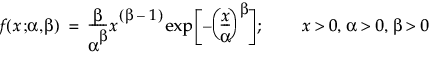
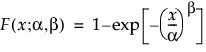
where α is a scale parameter, and β is a shape parameter. The Weibull distribution is particularly versatile because it reduces to an exponential distribution when β = 1. An alternative parameterization commonly used in the literature and in JMP is to use σ as the scale parameter and μ as the location parameter. These are easily converted to an α and β parameterization using the following definitions:

and

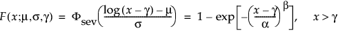
The pdf and the cdf of the Weibull distribution are also expressed as a log-transformed smallest extreme value distribution (SEV). This uses a location scale parameterization, with μ = log(α) and σ = 1/β,
where

and

are the pdf and cdf, respectively, for the standardized smallest extreme value (μ = 0, σ = 1) distribution.
Loglogistic
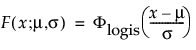
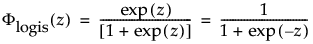
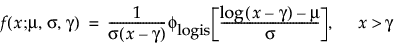
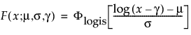
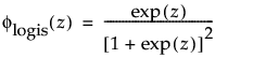
The pdf of the loglogistic distribution is similar in shape to the lognormal distribution but has heavier tails. It is often used to model data exhibiting non-monotonic hazard functions, such as cancer mortality and financial wealth. The loglogistic pdf and cdf are:
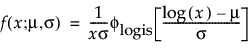
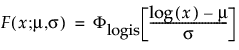
where
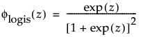
and

are the pdf and cdf, respectively, for the standardized logistic or logis distribution(μ = 0, σ = 1).
Fréchet
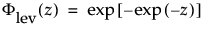
The Fréchet distribution is known as a log-largest extreme value distribution or sometimes as a Fréchet distribution of maxima when it is parameterized as the reciprocal of a Weibull distribution. This distribution is commonly used for financial data. The pdf and cdf are:
and are more generally parameterized as follows:
where
and

are the pdf and cdf, respectively, for the standardized largest extreme value LEV(μ = 0, σ = 1) distribution.
Normal
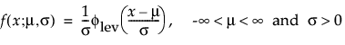
The normal distribution is the most widely used distribution in most areas of statistics because of its relative simplicity and the ease of applying the central limit theorem. However, it is rarely used in reliability. It is most useful for data where μ > 0 and the coefficient of variation (σ / μ) is small. Because the hazard function increases with no upper bound, it is particularly useful for data exhibiting wear-out failure. Examples include incandescent light bulbs, toaster heating elements, and mechanical strength of wires. The pdf and cdf are:
where

and
are the pdf and cdf, respectively, for the standardized normal, or nor(μ = 0, σ = 1) distribution.
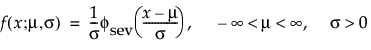
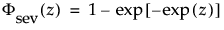
Smallest Extreme Value (SEV)
This non-symmetric (left-skewed) distribution is useful in two cases. The first case is when the data indicate a small number of weak units in the lower tail of the distribution (the data indicate the smallest number of many observations). The second case is when σ is small relative to μ, because probabilities of being less than zero, when using the SEV distribution, are small. The smallest extreme value distribution is useful to describe data whose hazard rate becomes larger as the unit becomes older. Examples include human mortality of the aged and rainfall amounts during a drought. This distribution is sometimes referred to as a Gumbel distribution. The pdf and cdf are:

where

and
are the pdf and cdf, respectively, for the standardized smallest extreme value, SEV(μ = 0, σ = 1) distribution.
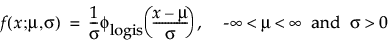
Logistic
The logistic distribution has a shape similar to the normal distribution, but with longer tails. The logistic distribution is often used to model life data when negative failure times are not an issue. Logistic regression models for a binary or ordinal response assume the logistic distribution as the latent distribution. The pdf and cdf are:
where

and
are the pdf and cdf, respectively, for the standardized logistic or logis distribution (μ = 0, σ = 1).
Largest Extreme Value (LEV)
This right-skewed distribution can be used to model failure times if σ is small relative to μ > 0. This distribution is not commonly used in reliability but is useful for estimating natural extreme phenomena, such as a catastrophic flood heights or extreme wind velocities. The pdf and cdf are:

where

and

are the pdf and cdf, respectively, for the standardized largest extreme value LEV(μ = 0, σ = 1) distribution.
Exponential
Both one- and two-parameter exponential distributions are used in reliability. The pdf and cdf for the two-parameter exponential distribution are:
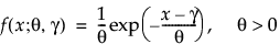
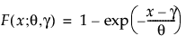
where θ is a scale parameter and γ is both the threshold and the location parameter. Reliability analysis frequently uses the one-parameter exponential distribution, with γ = 0. The exponential distribution is useful for describing failure times of components exhibiting wear-out far beyond their expected lifetimes. This distribution has a constant failure rate, which means that for small time increments, failure of a unit is independent of the unit’s age. The exponential distribution should not be used for describing the life of mechanical components that can be exposed to fatigue, corrosion, or short-term wear. This distribution is, however, appropriate for modeling certain types of robust electronic components. It has been used successfully to describe the life of insulating oils and dielectric fluids (Nelson 1990, p. 53).
Log Generalized Gamma (LogGenGamma)
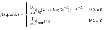
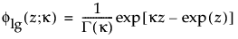
The log generalized gamma distribution contains the SEV, LEV, and Normal. The pdf and cdf are:
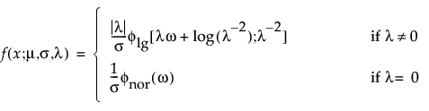
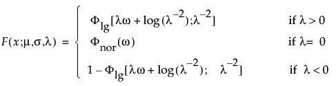
where −∞ < x < ∞, ω = [x – μ]/σ, and

Note that

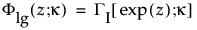
are the pdf and cdf, respectively, for the log-gamma variable and κ > 0 is a shape parameter. The standardized distributions above are dependent upon the shape parameter κ.
Note: In JMP, the shape parameter, λ, for the generalized gamma distribution is bounded between [-12,12] to provide numerical stability.
Extended Generalized Gamma (GenGamma)
The extended generalized gamma distribution can include many other distributions as special cases, such as the generalized gamma, Weibull, lognormal, Fréchet, gamma, and exponential. It is particularly useful for cases with little or no censoring. This distribution has been successfully modeled for human cancer prognosis. The pdf and cdf are:
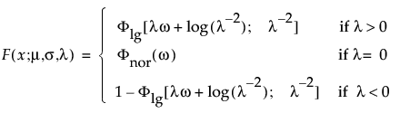
where x > 0, ω = [log(x) – μ]/σ, and

Note that

are the pdf and cdf, respectively, for the standardized log-gamma variable and κ > 0 is a shape parameter.
The standardized distributions above are dependent upon the shape parameter κ. Meeker and Escobar (1998, ch. 5) give a detailed explanation of the extended generalized gamma distribution.
Note: In JMP, the shape parameter, λ, for the generalized gamma distribution is bounded between [-12,12] to provide numerical stability.
Distributions with Threshold Parameters
Threshold Distributions are log-location-scale distributions with threshold parameters. Some of the distributions above are generalized by adding a threshold parameter, denoted by γ. The addition of this threshold parameter shifts the left endpoint of the distribution away from 0. Threshold parameters are sometimes called shift, minimum, or guarantee parameters because all units survive at least until threshold time. Note that while adding a threshold parameter shifts the distribution on the time axis, the shape, and spread of the distribution are not affected. Threshold distributions are useful for fitting moderately to heavily shifted distributions. The general forms for the pdf and cdf of a log-location-scale threshold distribution are:
where φ and Φ are the pdf and cdf, respectively, for the specific distribution. Examples of specific threshold distributions are shown below for the Weibull, lognormal, Fréchet, and loglogistic distributions, where, respectively, the SEV, Normal, LEV, and logis pdfs and cdfs are appropriately substituted.
Note: If the smallest observation is a failure (not censored), JMP creates a small interval around the point and treats the observation as interval censored. This padding around the failure bounds the log-likelihood function and improves estimation. If the smallest observation is censored, then no extra padding is added to the observation.
TH Weibull
The pdf and cdf of the three-parameter Weibull distribution are:
where μ =log(α), and σ= 1/β and where
and

are the pdf and cdf, respectively, for the standardized smallest extreme value, SEV(μ = 0, σ = 1) distribution.
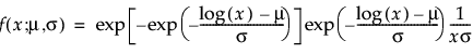
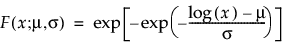
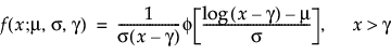
TH Lognormal
The pdf and cdf of the three-parameter lognormal distribution are:
where
and
are the pdf and cdf, respectively, for the standardized normal, or N(μ = 0, σ = 1) distribution.
TH Fréchet
The pdf and cdf of the three-parameter Fréchet distribution are:
where

and
are the pdf and cdf, respectively, for the standardized largest extreme value LEV(μ = 0, σ = 1) distribution.
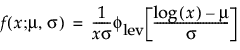
TH Loglogistic
The pdf and cdf of the three-parameter loglogistic distribution are:
where
and

are the pdf and cdf, respectively, for the standardized logistic or logis distribution (μ = 0, σ = 1).
Distributions for Defective Subpopulations
In reliability experiments, there are times when only a fraction of the population has a particular defect leading to failure. Because all units are not susceptible to failure, using the regular failure distributions is inappropriate and might produce misleading results. Use the DS distribution options to model failures that occur on only a subpopulation. The following DS distributions are available:
• DS Lognormal
• DS Weibull
• DS Loglogistic
• DS Fréchet
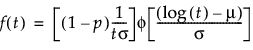
The pdf and cdf for defective subpopulation distributions are as follows:
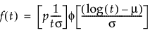
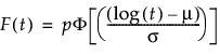
where:
p is the defective subpopulation fraction
t is the time of measurement for the lifetime event
μ and σ are estimated by calculating the usual maximum likelihood estimations using the pdf and cdf of the corresponding defective subpopulation
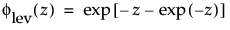
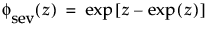
φ(z) and Φ(z) are the density and cumulative distribution function, respectively, for a standard distribution. For example, for a Weibull distribution,
φ(z) = exp(z-exp(z)) and Φ(z) = 1 - exp(-exp(z)).
See Tobias and Trindad (2012, p. 321) for more information about defective subpopulation models.
The defective subpopulation model is also known as a limited failure population model in Meeker and Escobar (1998, ch. 11).
Zero-Inflated Distributions
Zero-inflated distributions are used when some proportion (p) of the data fail at t = 0. When the data contain more zeros than expected by a standard model, the number of zeros is inflated. When the time-to-event data contain zero as the minimum value in the Life Distribution platform, four zero-inflated distributions are available. These distributions include:
• Zero-Inflated Lognormal (ZI Lognormal)
• Zero-Inflated Weibull (ZI Weibull)
• Zero-Inflated Loglogistic (ZI Loglogistic)
• Zero-Inflated Fréchet (ZI Fréchet)
The pdf and cdf for zero-inflated distributions are as follows:
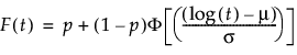
where:
p is the proportion of zero data values,
t is the time of measurement for the lifetime event,
μ and σ are estimated by calculating the usual maximum likelihood estimations after removing zero values from the original data,
φ(z) and Φ(z) are the density and cumulative distribution function, respectively, for a standard distribution. For example, for a Weibull distribution,
φ(z) = exp(z-exp(z)) and Φ(z) = 1 - exp(-exp(z)).
See Lawless (2003, p. 34) for more information about zero-inflated distributions. Substitute p = 1 - p and S1(t) = 1 - Φ(t) to obtain the form shown above.
See Tobias and Trindade (1995, p. 232) for more information about reliability distributions. This reference gives the general form for mixture distributions. Using the parameterization in Tobias and Trindade, the form above can be found by substituting α = p, Fd(t) = 1, and FN(t) = Φ(t).
Prior Distributions for Bayesian Estimation
The following distributions are available for Location Scale Priors:
• Normal/Lognormal, with hyperparameters Location (mu) and Scale (sigma). For a definition, see Lognormal and Normal.
• Uniform, with hyperparameters Low and End, which define the support of a Uniform distribution.
• Gamma, with hyperparameters Shape and Scale. The k/theta parameterization and the probability density function is used.
• Point Mass, with hyperparameter Location. This is a degenerated prior; there is only one possible value for the parameter that we are assigning a prior distribution to. The only possible value equals the value that is entered to this Location hyperparameter.
The following distributions are available for Quantile Parameter Priors:
• Normal/Lognormal, with a 99% probability range, specifies the prior distribution using the 0.005 and 0.995 percentiles of the distribution. JMP backs out the mu and sigma.
• Uniform, with hyperparameters Lower and Upper Limits, which define the support of a Uniform distribution.
• Log-Uniform, with Lower (a) and Upper (b) Limits. This distribution is uniform on the log scale between Log(a) and Log(b).
• Point Mass, with hyperparameter Location. This is a degenerated prior; there is only one possible value for the parameter that we are assigning a prior distribution to. The only possible value equals the value that is entered to this Location hyperparameter.
The following distributions are available for Failure Probability Priors:
• Beta, characterized by the probability density function.
– Specify the Beta prior using estimates and error percentages (mean and variance). The mean equals the number entered in to the Estimate, and the variance equals (Error Percentage / 100 * Estimate)^2.
– Specify the Beta prior using 0.005 and 0.995 percentiles of the distribution. JMP backs out the hyperparameters.